Checks and PCA
For manuscript: Neurogenomic landscape of male cooperative behavior in a wild bird
Last Substantive change December 2023
Last Knit “2024-01-05”
Here, I take the filtered dataset from the QC process, and run a whole brain analysis, as well as individual tissue analysis in the next markdown. Here, I also explore the relationships between our explanatory variables.
key<- read.csv("../data_filtered/data_key_Parsed_ReplicatesRemoved.csv")
behav<- read.csv("../data_unfiltered/PIPFIL_T_and_behav_data.csv")
rownames(key)<- key$X

key$Color_ID<- sub("/","", key$Color_ID)
key<- plyr::rename(key, replace=c("Color_ID"="colorID"))
behav$status<- plyr::revalue(behav$status, c("floa"="floater", "terr"="territorial"))
key_behav<- merge(key, behav, by="colorID")
key_behav<- key_behav[!is.na(key_behav$last_behav),]


#create a data.frame with all of the observations.
not_in_behav<- key[!key$X %in% key_behav$X,]
cols_not_key<- colnames(key_behav)[!colnames(key_behav) %in% colnames(key)]
cols_not_key_df<- data.frame(matrix(NA, nrow = nrow(not_in_behav), ncol = length(cols_not_key)))
colnames(cols_not_key_df)<- cols_not_key
not_in_behav<- cbind(not_in_behav, cols_not_key_df)

key_behav<- rbind(key_behav, not_in_behav)

rownames(key_behav)<- key_behav$X


key_behav$Tissue<- factor(key_behav$Tissue, levels=c("GON","PIT","VMH","AH","PVN","POM","ICO","GCT","AI","TNA","LS", "BSTm"))
key_behav<- key_behav[order(rownames(key_behav)),]
key_behav$Class<- as.factor(key_behav$Class)
key_behav$Class<- revalue(key_behav$Class, replace=c("SCB floater"="Predefinitive floater", "DCB floater "="Definitive floater", "DCB territorial"="Territorial"))
key_behav$Class<- factor(key_behav$Class, levels=c("Predefinitive floater", "Definitive floater", "Territorial"))
rownames(key_behav)<- key_behav$sampleID
key_behav<- key_behav[order(key_behav$sampleID),]
key_behav$Year<- as.factor(key_behav$Year)
key_behav$Batch<- as.factor(key_behav$Batch)
key_behav$Status<- as.factor(key_behav$Status)

key_behav_unique<- key_behav[!duplicated(key_behav$colorID),]


#read the raw count data
data<- read.csv("../data_filtered/data_RawCounts_all_ReplicatesRemoved_antisense_V2.csv")

rownames(data)<- data$X
data$X<- NULL

### Gene Ontology

go_key<- read.csv("../GO_annotations/Maggies_annotations_modifiedR.csv")
go_key<- plyr::rename(go_key, replace=c("GeneID"="gene"))

go_terms<- read.csv("../GO_annotations/pfil_GO_key_raw.csv")
go_terms<- plyr::rename(go_terms, replace=c("GeneID"="gene"))
go2gene_bp<- go_terms[which(go_terms$Aspect=="P"),c("GO_ID", "gene")]
go2gene_mf<- go_terms[which(go_terms$Aspect=="F"),c("GO_ID", "gene")]
go_obo<- read.csv("../GO_annotations/ontology_obo_out.csv")
go_obo<- plyr::rename(go_obo, replace=c("id"="GO_ID"))
go2name_bp<- go_obo[which(go_obo$namespace=="biological_process"),c("GO_ID", "name")]
go2name_mf<- go_obo[which(go_obo$namespace=="molecular_function"),c("GO_ID", "name")]


genes_key<- read.csv("../GO_annotations/Maggies_annotations_modifiedR.csv")
genes_key<- plyr::rename(genes_key, replace=c("GeneID"="gene"))
genes_key$gene[genes_key$gene=="LOC113993669"] <- "CYP19A1"
genes_key$gene[genes_key$gene=="LOC113983511"] <- "OXT"
genes_key$gene[genes_key$gene=="LOC113983498"] <- "AVP"
genes_key$gene[genes_key$gene=="LOC113982601"] <- "AVPR2"
data_genes<- data.frame(gene=rownames(data))
genes_key<- merge(data_genes, genes_key, by="gene", all.x=TRUE)
#genes_key<- genes_key[which(grepl("LOC[0-9]+",genes_key$gene)),]

genes_key$display_gene_ID<- ifelse(grepl("LOC[0-9]+", genes_key$gene) & !grepl("LOC[0-9]+",genes_key$best_anno) & !is.na(genes_key$best_anno), paste0(genes_key$gene," (",genes_key$best_anno,")"), as.character(genes_key$gene))
genes_key<- genes_key[,c("gene","best_anno","display_gene_ID")]
1 Exploration of the behavioural data
We were concerned about the signal from the last few days outweighing the gene-expression signal from their overall phenotype, so we will explore how different these measures are from eachother.
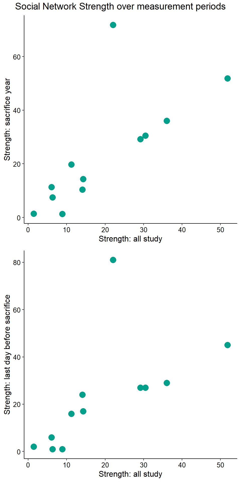
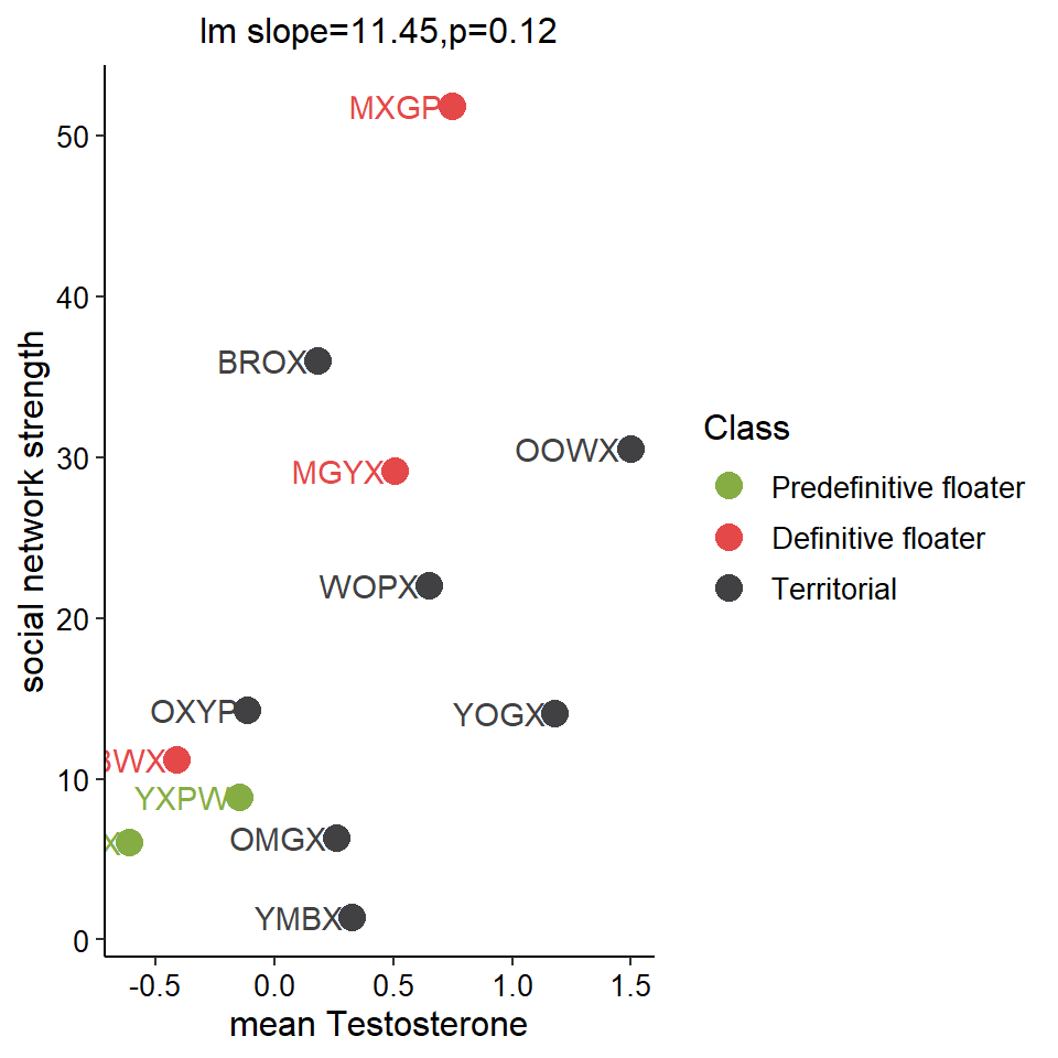
1.1 Associations between variables
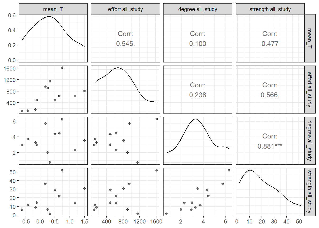
Given the significant relationship between degree and strength, I will only keep one of these variables - the strength. This was the most repeatable of the two sociality variables in Ryder et al. (2020).
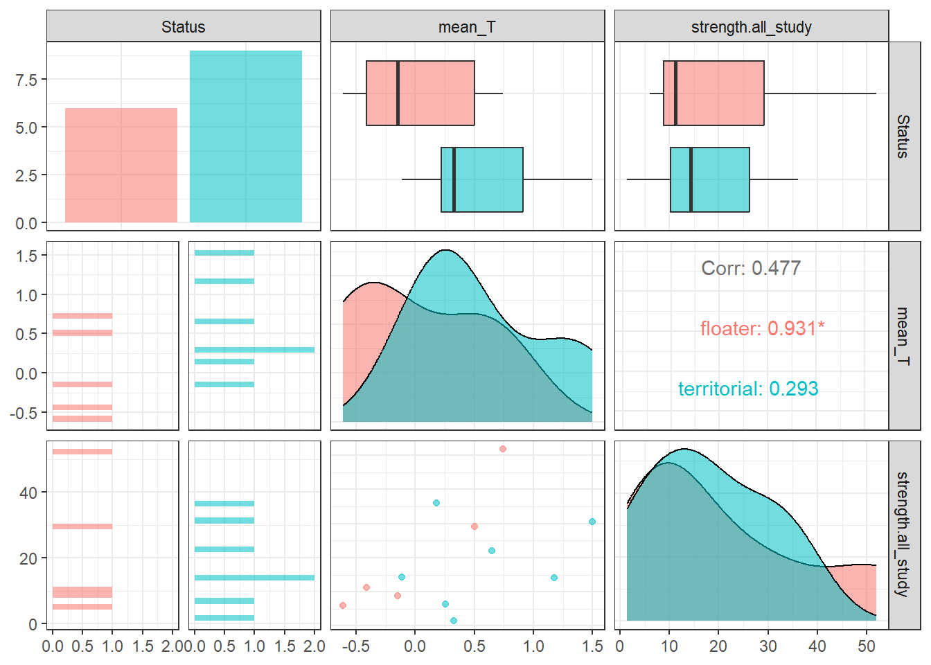
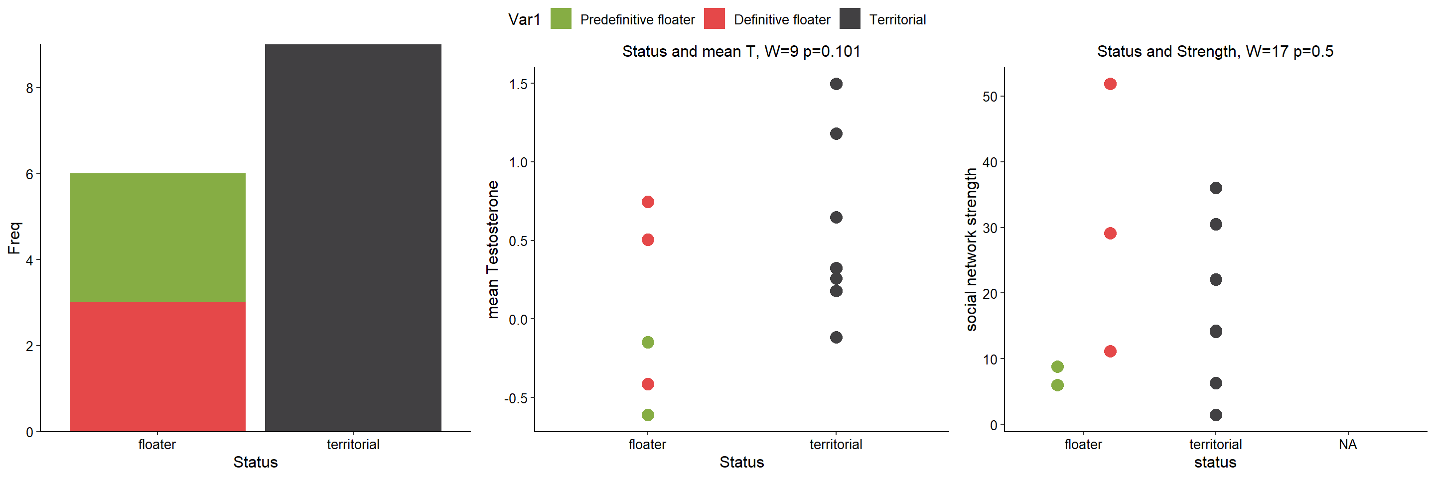
All significance tests cited in the figure above are based on just territorial and floater, but colour-coded according to plumage*status.
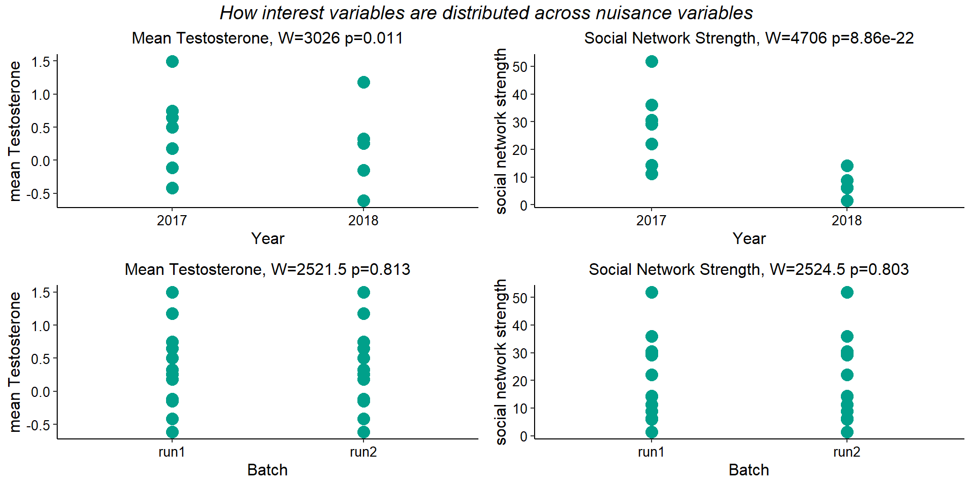
1.2 Nuisance variables
In the previous QC exploration I found substantial DEGs according to collection Year and Sequencing Batch. Here we explore how the continuous variables are distributed across sampling years. The tests find there is a difference in the medians between years for both our interest traits.
2 All tissues PCA
Plotting all the tissues
all_data<- data

start<- nrow(all_data)
#remove genes with avg read counts <20
all_data$avg_count<- apply(all_data, 1, mean)
all_data<- all_data[all_data$avg_count>20,]
all_data$avg_count<-NULL


#remove genes where >50% of samples have 0 gene expression
all_data$percent_0<- apply(all_data, 1, function(x)length(x[x==0]))
thresh<- ncol(all_data)/2
all_data<- all_data[all_data$percent_0<=thresh,]
all_data$percent_0<-NULL
nrow(all_data)
FALSE [1] 14414
FALSE [1] "Batch"
FALSE [1] "Tissue"
FALSE [1] "Status"
FALSE [1] "Year"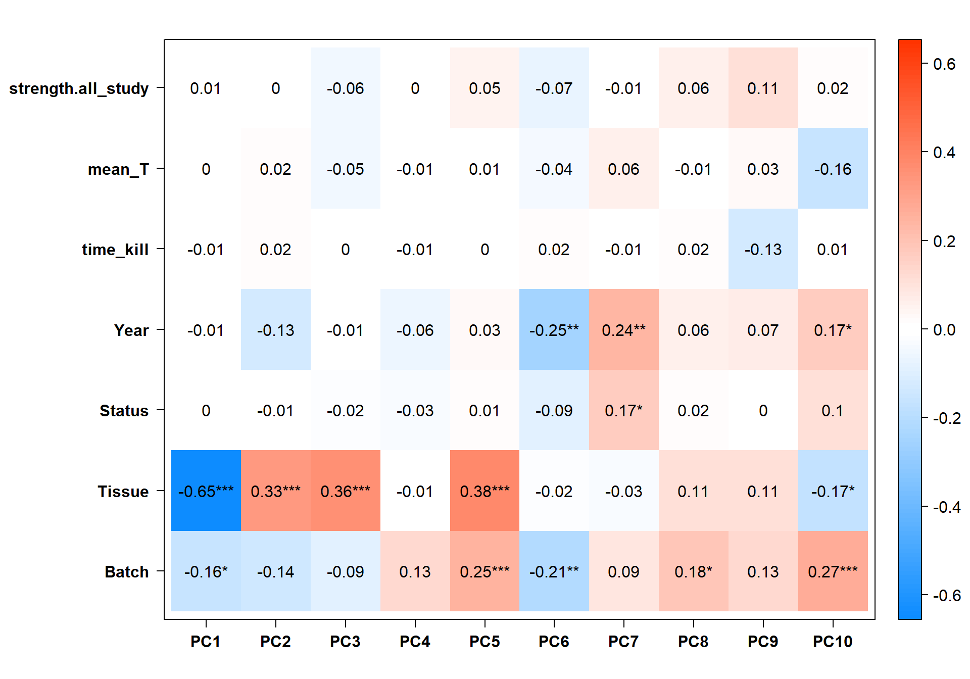
Based on these results it seems like PC7 is associated with social Status. Let’s explore this PC further.
FALSE [1] "Batch"
FALSE [1] "Tissue"
FALSE [1] "Status"
FALSE [1] "Year"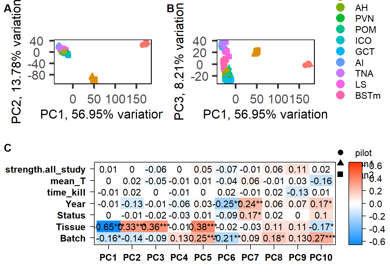
#library(nlme)


test<- data.frame(PC7=p$rotated$PC7)
test<- cbind(test, key_behav)


m0<- lm(PC7 ~ 1, data=test)

m01<- lm(PC7 ~ Year, data=test)
m01.aov<- Anova(m01, type=2)

m02<- lm(PC7 ~ Year + Tissue, data=test)
m02.aov<- Anova(m02, type=2)
m02.aov
FALSE Anova Table (Type II tests)
FALSE
FALSE Response: PC7
FALSE Sum Sq Df F value Pr(>F)
FALSE Year 2216.1 2 28.775 2.255e-11 ***
FALSE Tissue 5887.0 11 13.899 < 2.2e-16 ***
FALSE Residuals 6045.6 157
FALSE ---
FALSE Signif. codes: 0 '***' 0.001 '**' 0.01 '*' 0.05 '.' 0.1 ' ' 1m02.vif<- sum(vif(m02)[,1])
m1<- lm(PC7~ Year + Tissue + Status,data=test)
m1.aov<- Anova(m1, type=2)
m1.aovFALSE Anova Table (Type II tests)
FALSE
FALSE Response: PC7
FALSE Sum Sq Df F value Pr(>F)
FALSE Year 2103.1 2 28.3853 3.066e-11 ***
FALSE Tissue 5851.9 11 14.3607 < 2.2e-16 ***
FALSE Status 266.5 1 7.1946 0.0081 **
FALSE Residuals 5779.0 156
FALSE ---
FALSE Signif. codes: 0 '***' 0.001 '**' 0.01 '*' 0.05 '.' 0.1 ' ' 1m1.vif<- sum(vif(m1)[,1])
m2<- lm(PC7~ Year + Tissue * Status,data=test,contrasts=list(Tissue=contr.sum, Status=contr.sum))
m2.aov<- Anova(m2, type=3)
m2.aovFALSE Anova Table (Type III tests)
FALSE
FALSE Response: PC7
FALSE Sum Sq Df F value Pr(>F)
FALSE (Intercept) 1778.0 1 47.8645 1.358e-10 ***
FALSE Year 2030.9 2 27.3355 8.440e-11 ***
FALSE Tissue 5792.6 11 14.1759 < 2.2e-16 ***
FALSE Status 294.5 1 7.9272 0.005548 **
FALSE Tissue:Status 392.6 11 0.9609 0.484768
FALSE Residuals 5386.4 145
FALSE ---
FALSE Signif. codes: 0 '***' 0.001 '**' 0.01 '*' 0.05 '.' 0.1 ' ' 1FALSE Anova Table (Type II tests)
FALSE
FALSE Response: PC7
FALSE Sum Sq Df F value Pr(>F)
FALSE Year 2030.9 2 27.3355 8.44e-11 ***
FALSE Tissue 5851.9 11 14.3211 < 2.2e-16 ***
FALSE Status 266.5 1 7.1748 0.008247 **
FALSE Tissue:Status 392.6 11 0.9609 0.484768
FALSE Residuals 5386.4 145
FALSE ---
FALSE Signif. codes: 0 '***' 0.001 '**' 0.01 '*' 0.05 '.' 0.1 ' ' 1m3<- lm(PC7~ Tissue + Status + Tissue:Status,data=test,contrasts=list(Tissue=contr.sum, Status=contr.sum))
m3.aov<- Anova(m3, type=3)
m3.aovFALSE Anova Table (Type III tests)
FALSE
FALSE Response: PC7
FALSE Sum Sq Df F value Pr(>F)
FALSE (Intercept) 14.4 1 0.2858 0.593714
FALSE Tissue 5361.8 11 9.6603 5.32e-13 ***
FALSE Status 404.1 1 8.0096 0.005304 **
FALSE Tissue:Status 464.8 11 0.8375 0.602960
FALSE Residuals 7417.3 147
FALSE ---
FALSE Signif. codes: 0 '***' 0.001 '**' 0.01 '*' 0.05 '.' 0.1 ' ' 1FALSE Anova Table (Type II tests)
FALSE
FALSE Response: PC7
FALSE Sum Sq Df F value Pr(>F)
FALSE Tissue 5421.3 11 9.7676 3.887e-13 ***
FALSE Status 379.5 1 7.5214 0.006855 **
FALSE Tissue:Status 464.8 11 0.8375 0.602960
FALSE Residuals 7417.3 147
FALSE ---
FALSE Signif. codes: 0 '***' 0.001 '**' 0.01 '*' 0.05 '.' 0.1 ' ' 1m4<- lm(PC7~ Tissue + Status,data=test)
m4.aov<- Anova(m4, type=2)
m4.vif<- sum(vif(m4)[,1])
models<- c("~ 1", "~ Year", "~ Year + Tissue","~ Year + Tissue + Status" , "~ Year + Tissue + Status + Tissue:Status","~ Tissue + Status + Tissue:Status", "~ Tissue + Status")
aic=signif(c(AIC(m0),AIC(m01),AIC(m02),AIC(m1),AIC(m2),AIC(m3),AIC(m4)),4)
deltaAIC<- signif(c(NA,aic[1]-aic[2],aic[1]-aic[3], aic[1]-aic[4],aic[1]-aic[5],aic[1]-aic[6],aic[1]-aic[7]),3)
batch_p<- signif(c(NA, m01.aov$'Pr(>F)'[1],m02.aov$'Pr(>F)'[1],m1.aov$'Pr(>F)'[1],m2.aov$'Pr(>F)'[2],NA,NA),2)
e_p<- signif(c(NA, NA,NA,m1.aov$'Pr(>F)'[3],m2.aov$
'Pr(>F)'[3],m3.aov$
'Pr(>F)'[2],m4.aov$'Pr(>F)'[2]),2)
sumVIF<- round(c(NA,NA,m02.vif, m1.vif,m2.vif, m3.vif, m4.vif),0)
ms<- data.frame(models,aic, deltaAIC,batch_p,e_p, sumVIF)
ms<- ggtexttable(ms,theme = ttheme(base_size = 6,padding=unit(c(4,10),"pt")),rows=NULL)
pc7test<- cbind(m1.aov, c(eta_squared(m1.aov)$Eta2_partial,NA))
colnames(pc7test)[5]<- "eta^2"
summary(m1)FALSE
FALSE Call:
FALSE lm(formula = PC7 ~ Year + Tissue + Status, data = test)
FALSE
FALSE Residuals:
FALSE Min 1Q Median 3Q Max
FALSE -33.893 -3.689 0.468 3.619 15.790
FALSE
FALSE Coefficients:
FALSE Estimate Std. Error t value Pr(>|t|)
FALSE (Intercept) -8.7256 1.8534 -4.708 5.49e-06 ***
FALSE Year2017 9.9678 1.3420 7.427 6.79e-12 ***
FALSE Year2018 8.7427 1.4104 6.199 4.86e-09 ***
FALSE TissuePIT -0.4707 2.3458 -0.201 0.84122
FALSE TissueVMH 4.1733 2.1519 1.939 0.05426 .
FALSE TissueAH -6.4939 2.4057 -2.699 0.00771 **
FALSE TissuePVN -5.9021 2.3458 -2.516 0.01288 *
FALSE TissuePOM -1.5015 2.1519 -0.698 0.48636
FALSE TissueICO 4.2951 2.2295 1.926 0.05586 .
FALSE TissueGCT -5.1958 2.2836 -2.275 0.02425 *
FALSE TissueAI 11.1688 2.2281 5.013 1.44e-06 ***
FALSE TissueTNA -11.9698 2.1519 -5.562 1.13e-07 ***
FALSE TissueLS 1.5645 2.1886 0.715 0.47579
FALSE TissueBSTm 1.9793 2.1519 0.920 0.35909
FALSE Statusterritorial 2.5403 0.9471 2.682 0.00810 **
FALSE ---
FALSE Signif. codes: 0 '***' 0.001 '**' 0.01 '*' 0.05 '.' 0.1 ' ' 1
FALSE
FALSE Residual standard error: 6.086 on 156 degrees of freedom
FALSE Multiple R-squared: 0.5786, Adjusted R-squared: 0.5407
FALSE F-statistic: 15.3 on 14 and 156 DF, p-value: < 2.2e-16#pc5test<- summary(aov(test$PC5 ~ test$Year + test$Status))
pc5test_anova <- ggtexttable(signif(pc7test,2),theme = ttheme(base_size = 6,padding=unit(c(4,10),"pt")),rows=rownames(pc7test)) %>% tab_add_title(text = "PC7 ~ Year + Tissue + Status ", size=6, padding = unit(0.1, "line"))
e<-biplot(p, x="PC1",y="PC7", lab=NULL, colby="Tissue", shape="Status", legendPosition="right", title="") + peri_theme
f<-ggplot(test, aes(x=Tissue, y=PC7, colour=Status)) + geom_boxplot(outlier.colour = NA) + geom_point(position=dodge) + peri_theme + theme(legend.position="none") + scale_colour_manual(values=status_cols[2:3]) + theme(axis.text.x=element_text(angle=90))
g<- ggarrange(ggarrange(f,ggarrange(ms,pc5test_anova, nrow=2, labels=c("B","C")), ncol=2, labels=c("A")),c, ncol=1, nrow=2,labels=c("","D"))
g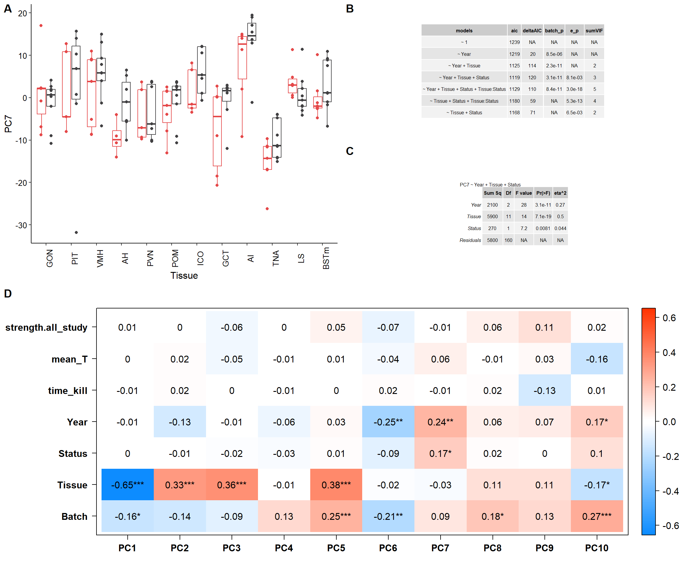
ggsave(filename="../PCA_results/figure_alltissues_PC7.pdf",plot=g, device="pdf",height =6 ,width=7.5, units="in",bg="white")
ggsave(filename="../PCA_results/figure_alltissues_PC7.png", plot=g,device="png",height =6 ,width=7.5, units="in", bg="white")
Let’s see what genes are associated with each principal component. See GitHub repository for larger version.
loadings<- p$loadings
loadings$gene<- rownames(loadings)
loadings<- merge(loadings, genes_key, by="gene")
plots<- list()
pcs<- paste0("PC",1:10)
for(i in pcs){
#i="PC2"
sub<- loadings[,c(i, "display_gene_ID","gene")]
sub<- sub[order(sub[,i]),]
top30<- rbind(head(sub,15), tail(sub,15))
top30$best_anno2<- factor(top30$display_gene_ID, levels=unique(top30$display_gene_ID[order(top30[,i],top30$display_gene_ID)]), ordered=TRUE)
top30$pos<- ifelse(top30[,i]<0, "neg", "pos")
plots[[i]]<-ggplot(top30, aes(x=best_anno2, y=top30[,i], fill=pos)) + geom_bar(stat="identity")+ peri_figure_supp + coord_flip() + labs(x="gene", y=paste(i,"loading")) + scale_fill_manual(values=c("#0D8CFF","#FF3300")) + theme(legend.position="none")
}
p<- ggarrange(plotlist=plots, ncol=5, nrow=2)
ggsave(filename="../PCA_results/figure_alltissue_loadings.pdf",p, device="pdf",height =8.5 ,width=16, units="in", bg="white")
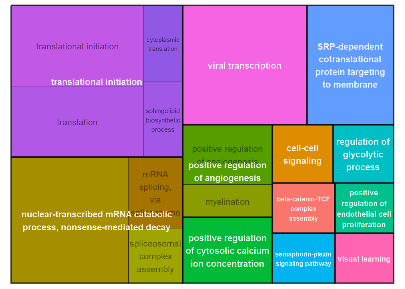
ggsave(filename="../PCA_results/figure_alltissue_loadings.png",p, device="png",height =8.5 ,width=16, units="in", bg="white")2.1 PC7 Gene Ontology
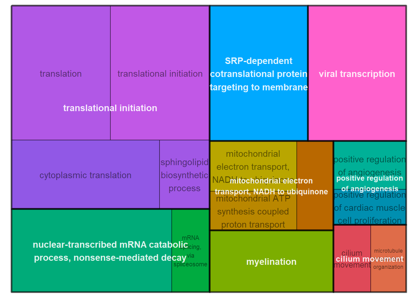
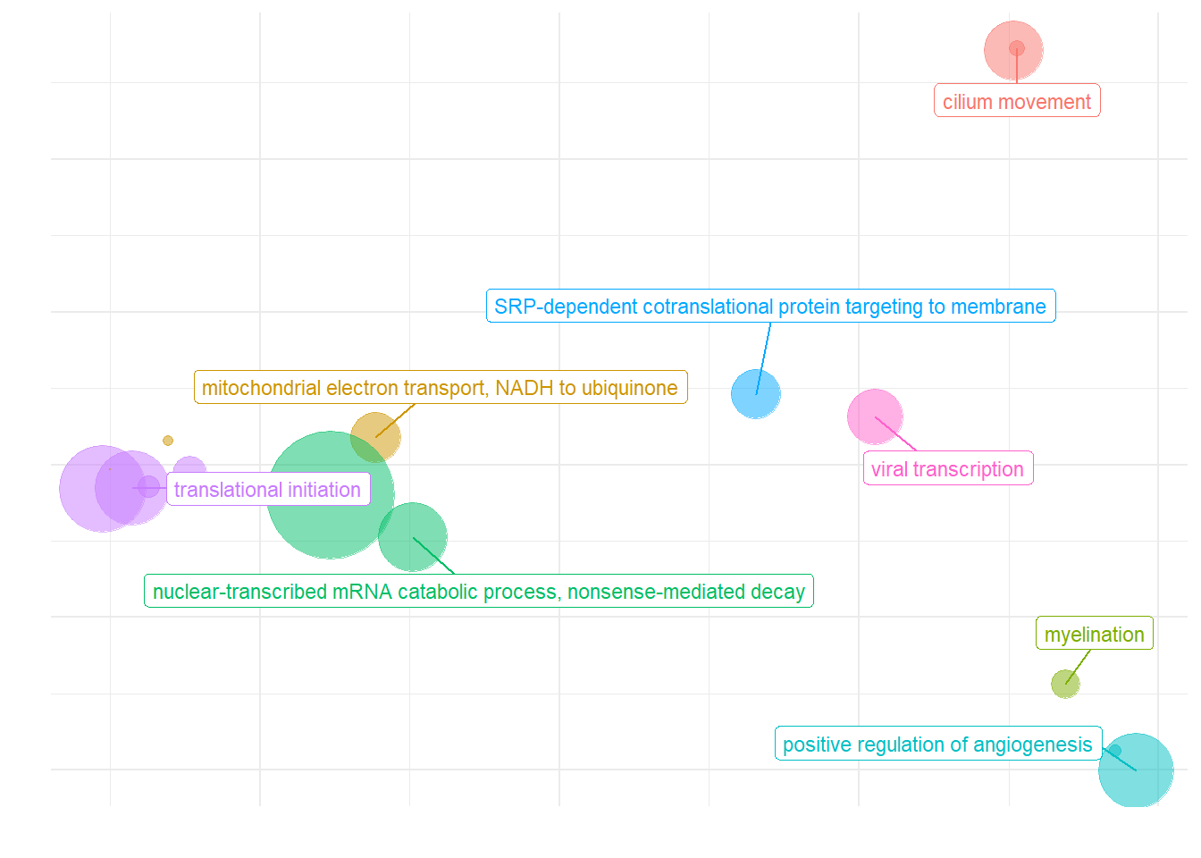
What are the gene ontology categories enriched in PC7?
res_go<- loadings[c("gene","PC7","best_anno")]
#res_go$logP<- -log(abs(res_go$PC5), 10)
#res_go$logP<- ifelse(res_go$PC5<0, -(res_go$logP), res_go$logP)
res_go<- res_go[order(res_go$PC7, decreasing=TRUE),]
geneList<- res_go$PC7
names(geneList)<- res_go$gene
y<- GSEA(geneList, TERM2GENE = go2gene_bp, TERM2NAME = go2name_bp)
y@result$Description<- ifelse(str_count(y@result$Description, '\\w+') >= 10,
gsub("(^[^\\s]+\\s[^\\s]+\\s[^\\s]+\\s[^\\s]+\\s[^\\s]+\\s[^\\s]+)\\s","\\1\n",y@result$Description, perl=TRUE),
ifelse(str_count(y@result$Description, '\\w+') >= 6,
gsub("(^[^\\s]+\\s[^\\s]+\\s[^\\s]+\\s[^\\s]+)\\s","\\1\n",y@result$Description, perl=TRUE),
as.character(y@result$Description)))
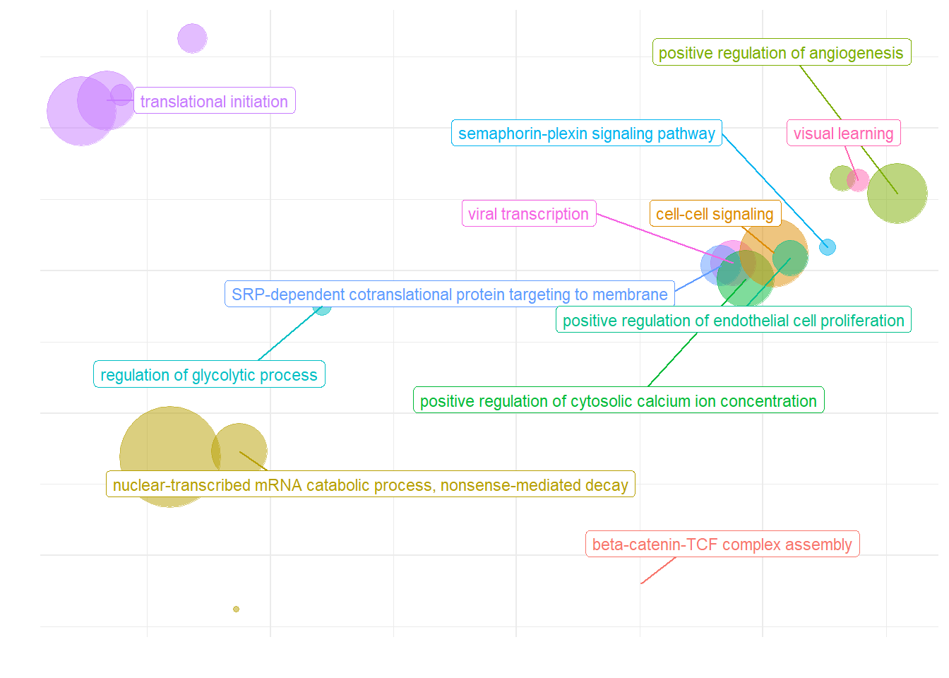
ridgeplot(y, fill="pvalue", showCategory=20) + peri_figure_supp + labs(title=paste0("Top 20 GO BP terms from GSEA\n in PC7 according"), x="direction scaled log10(p-value)") + scale_fill_viridis(option="G") + theme(legend.key.size=unit(3,"mm"))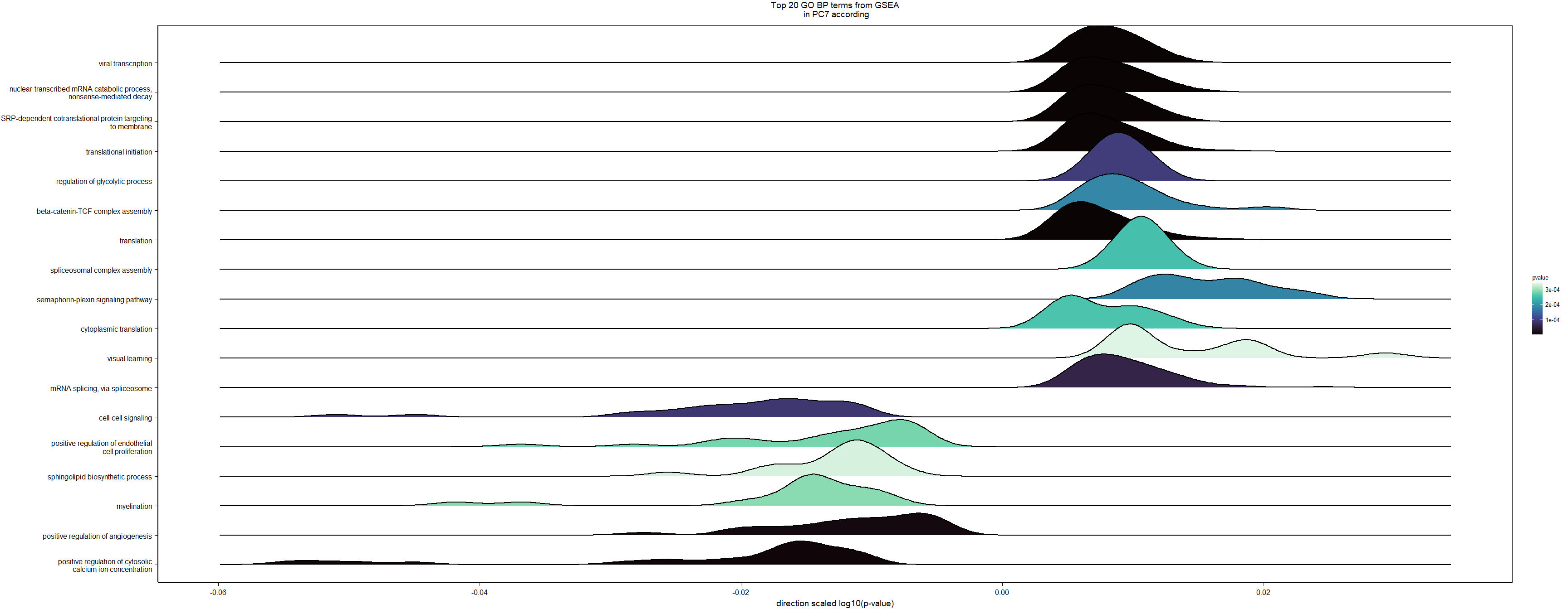
3 Wholebrain PCA
outliers=c("PFT2_POM_run1")

brain_behav<- subset(key_behav, Tissue!="GON")
brain_behav<- subset(brain_behav, Tissue!="PIT")
brain_behav<- brain_behav[!rownames(brain_behav) %in% outliers,]
brain_behav<- droplevels(brain_behav)


brain_data<- data[,colnames(data) %in% rownames(brain_behav)]

start<- nrow(brain_data)
#remove genes with avg read counts <20
brain_data$avg_count<- apply(brain_data, 1, mean)
brain_data<- brain_data[brain_data$avg_count>20,]
brain_data$avg_count<-NULL


#remove genes where >50% of samples have 0 gene expression
brain_data$percent_0<- apply(brain_data, 1, function(x)length(x[x==0]))
thresh<- ncol(brain_data)/2
brain_data<- brain_data[brain_data$percent_0<=thresh,]
brain_data$percent_0<-NULL
#13652 genes.
Looking for cohesive signatures across the whole brain. Overall, before this round of filtering for the brain dataset we have 16854 genes. After filtering we have 13653 genes. This final document is the result of lots of work in single tissues to determine outlier status that were identified in the QC process. We are excluding PFT2_POM_run1 because the analyses below indicated that it was an outlier within POM, other potentials identified in the QC process were not deemed outliers.
FALSE [1] "Batch"
FALSE [1] "Tissue"
FALSE [1] "Status"
FALSE [1] "Year"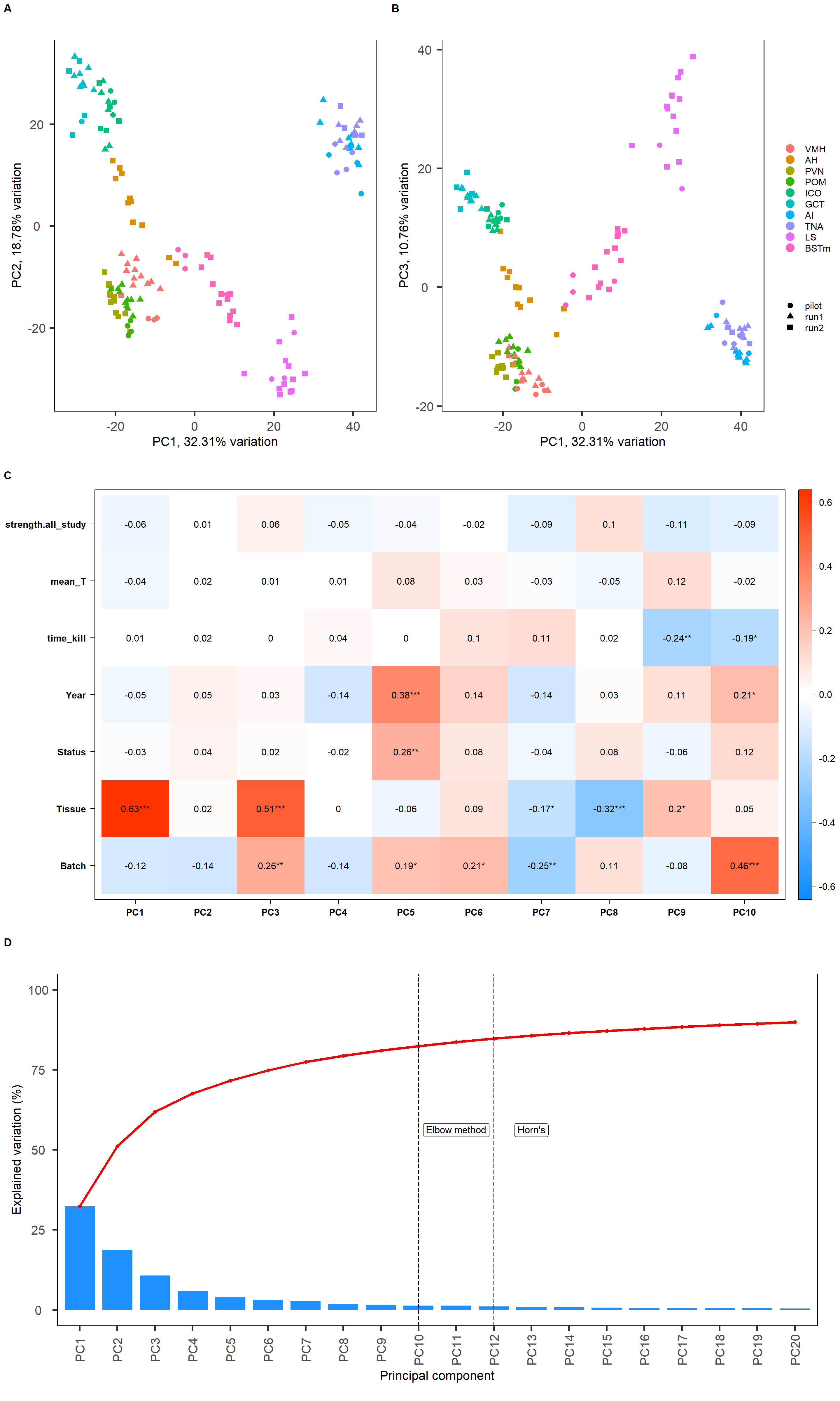
PC5 seems to be associated with our interest variables.
FALSE Anova Table (Type II tests)
FALSE
FALSE Response: PC5
FALSE           Sum Sq  Df F value    Pr(>F)
FALSE Year      3471.5   2 46.7499 5.050e-16 ***
FALSE Tissue    3266.2   9  9.7745 2.494e-11 ***
FALSE Residuals 4826.7 130
FALSE ---
FALSE Signif. codes:  0 '***' 0.001 '**' 0.01 '*' 0.05 '.' 0.1 ' ' 1
FALSE Anova Table (Type II tests)
FALSE
FALSE Response: PC5
FALSE Sum Sq Df F value Pr(>F)
FALSE Year 3271.1 2 48.888 < 2.2e-16 ***
FALSE Tissue 3255.2 9 10.811 2.109e-12 ***
FALSE Status 511.0 1 15.273 0.0001494 ***
FALSE Residuals 4315.8 129
FALSE ---
FALSE Signif. codes: 0 '***' 0.001 '**' 0.01 '*' 0.05 '.' 0.1 ' ' 1FALSE Anova Table (Type III tests)
FALSE
FALSE Response: PC5
FALSE Sum Sq Df F value Pr(>F)
FALSE (Intercept) 2925.0 1 87.0463 6.787e-16 ***
FALSE Year 3197.9 2 47.5846 6.082e-16 ***
FALSE Tissue 3305.1 9 10.9288 2.709e-12 ***
FALSE Status 551.4 1 16.4107 9.084e-05 ***
FALSE Tissue:Status 283.5 9 0.9373 0.4957
FALSE Residuals 4032.3 120
FALSE ---
FALSE Signif. codes: 0 '***' 0.001 '**' 0.01 '*' 0.05 '.' 0.1 ' ' 1FALSE Anova Table (Type III tests)
FALSE
FALSE Response: PC5
FALSE Sum Sq Df F value Pr(>F)
FALSE (Intercept) 44.2 1 0.7452 0.3897070
FALSE Tissue 2626.3 9 4.9238 1.225e-05 ***
FALSE Status 748.9 1 12.6365 0.0005391 ***
FALSE Tissue:Status 356.7 9 0.6687 0.7358179
FALSE Residuals 7230.2 122
FALSE ---
FALSE Signif. codes: 0 '***' 0.001 '**' 0.01 '*' 0.05 '.' 0.1 ' ' 1FALSE Anova Table (Type II tests)
FALSE
FALSE Response: PC5
FALSE Sum Sq Df F value Pr(>F)
FALSE Tissue 2565.2 9 4.8093 1.692e-05 ***
FALSE Status 711.4 1 12.0036 0.0007334 ***
FALSE Tissue:Status 356.7 9 0.6687 0.7358179
FALSE Residuals 7230.2 122
FALSE ---
FALSE Signif. codes: 0 '***' 0.001 '**' 0.01 '*' 0.05 '.' 0.1 ' ' 1FALSE Anova Table (Type II tests)
FALSE
FALSE Response: PC5
FALSE Sum Sq Df F value Pr(>F)
FALSE Tissue 2565.2 9 4.9213 1.086e-05 ***
FALSE Status 711.4 1 12.2832 0.0006261 ***
FALSE Residuals 7586.9 131
FALSE ---
FALSE Signif. codes: 0 '***' 0.001 '**' 0.01 '*' 0.05 '.' 0.1 ' ' 1FALSE
FALSE Call:
FALSE lm(formula = PC5 ~ Year + Tissue + Status, data = test)
FALSE
FALSE Residuals:
FALSE Min 1Q Median 3Q Max
FALSE -14.4015 -3.5505 0.1036 3.4221 12.6575
FALSE
FALSE Coefficients:
FALSE Estimate Std. Error t value Pr(>|t|)
FALSE (Intercept) -7.1246 1.8083 -3.940 0.000133 ***
FALSE Year2017 13.0110 1.3751 9.462 < 2e-16 ***
FALSE Year2018 12.5517 1.4441 8.692 1.39e-14 ***
FALSE TissueAH -16.8285 2.2893 -7.351 2.01e-11 ***
FALSE TissuePVN -7.8026 2.2324 -3.495 0.000650 ***
FALSE TissuePOM -3.9960 2.0793 -1.922 0.056838 .
FALSE TissueICO -1.7180 2.1192 -0.811 0.419039
FALSE TissueGCT -8.7007 2.1717 -4.006 0.000104 ***
FALSE TissueAI 0.2132 2.1175 0.101 0.919963
FALSE TissueTNA -9.9407 2.0450 -4.861 3.33e-06 ***
FALSE TissueLS -2.3957 2.0800 -1.152 0.251559
FALSE TissueBSTm -7.7393 2.0450 -3.785 0.000235 ***
FALSE Statusterritorial 3.8609 0.9879 3.908 0.000149 ***
FALSE ---
FALSE Signif. codes: 0 '***' 0.001 '**' 0.01 '*' 0.05 '.' 0.1 ' ' 1
FALSE
FALSE Residual standard error: 5.784 on 129 degrees of freedom
FALSE Multiple R-squared: 0.6026, Adjusted R-squared: 0.5656
FALSE F-statistic: 16.3 on 12 and 129 DF, p-value: < 2.2e-16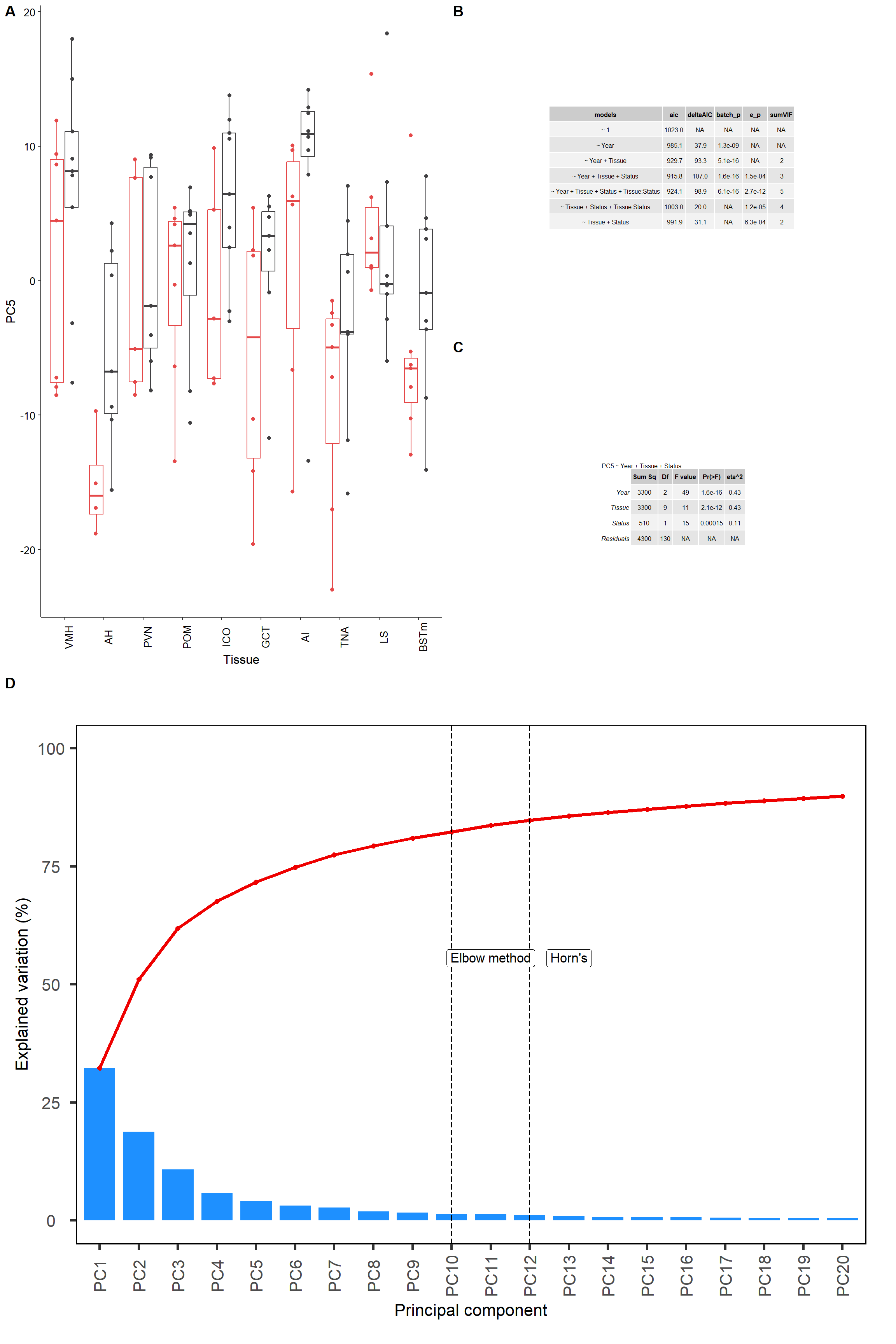
loadings<- p$loadings
loadings$gene<- rownames(loadings)
loadings<- merge(loadings, genes_key, by="gene")


plots<- list()
pcs<- paste0("PC",1:10)
for(i in pcs){
  #i="PC2"
  sub<- loadings[,c(i, "display_gene_ID","gene")]
  sub<- sub[order(sub[,i]),]
  top30<- rbind(head(sub,15), tail(sub,15))
  top30$best_anno2<- factor(top30$display_gene_ID, levels=unique(top30$display_gene_ID[order(top30[,i],top30$display_gene_ID)]), ordered=TRUE)
  top30$pos<- ifelse(top30[,i]<0, "neg", "pos")
  plots[[i]]<-ggplot(top30, aes(x=best_anno2, y=top30[,i], fill=pos)) + geom_bar(stat="identity")+  peri_figure_supp + coord_flip() + labs(x="gene", y=paste(i,"loading")) + scale_fill_manual(values=c("#0D8CFF","#FF3300")) + theme(legend.position="none")
}
ggarrange(plotlist=plots, ncol=5, nrow=2)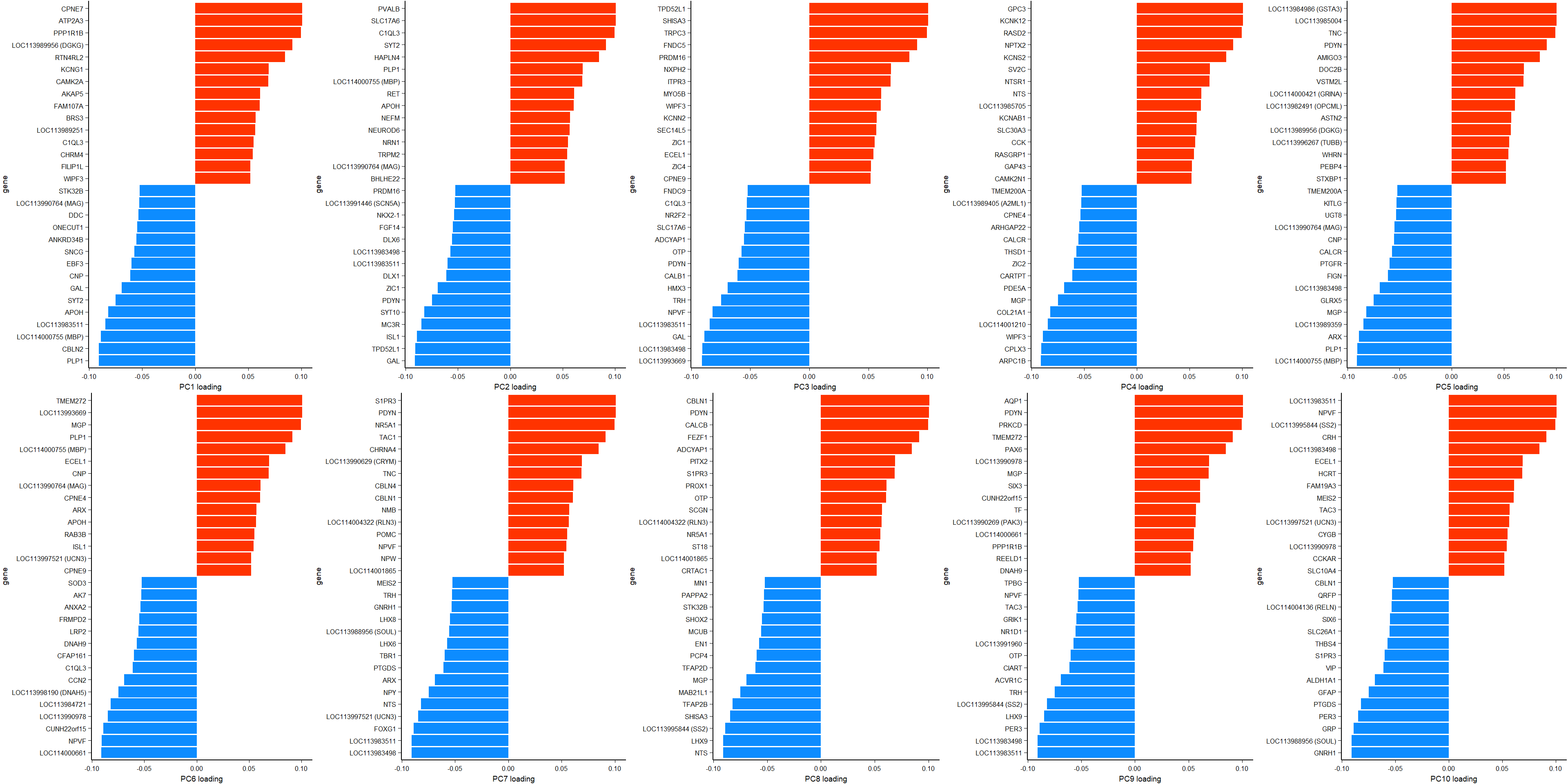
ggsave(filename="../PCA_results/figure_brain_loadings.pdf", device="pdf",height =8.5 ,width=16, units="in", bg="white")
ggsave(filename="../PCA_results/figure_brain_loadings.png", device="png",height =8.5 ,width=16, units="in", bg="white")
3.1 PC5 Gene Ontology
What are the gene ontology categories enriched in PC5?
res_go<- loadings[c("gene","PC5","best_anno")]
#res_go$logP<- -log(abs(res_go$PC5), 10)
#res_go$logP<- ifelse(res_go$PC5<0, -(res_go$logP), res_go$logP)
res_go<- res_go[order(res_go$PC5, decreasing=TRUE),]


geneList<- res_go$PC5
names(geneList)<- res_go$gene


y<- GSEA(geneList, TERM2GENE = go2gene_bp, TERM2NAME = go2name_bp)
ridgeplot(y) + scale_fill_viridis(direction=-1) + peri_theme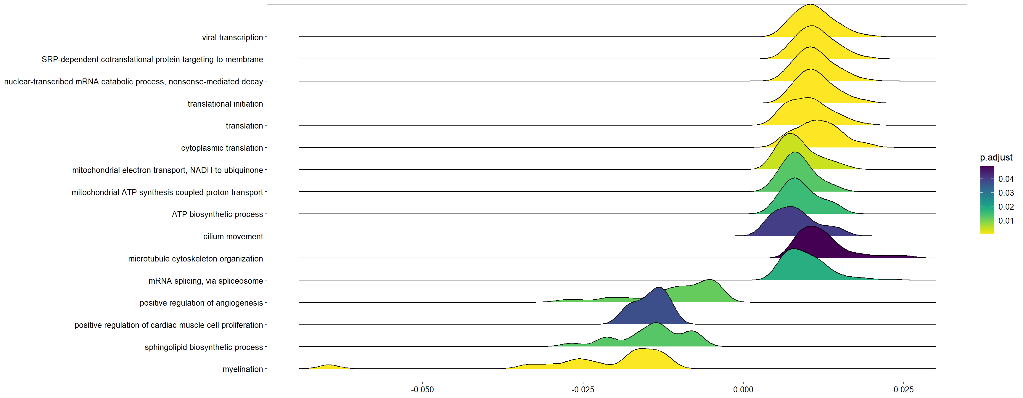
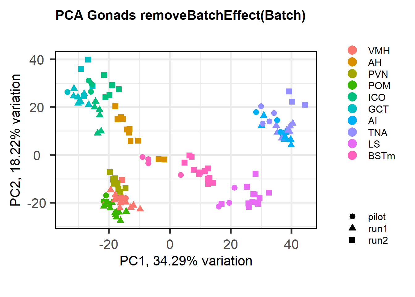
3.2 Batch Effects
What happens if I use batch effect exclusion on the whole brain? This way I wouldn’t have to use single tissue
FALSE [1] "Batch"
FALSE [1] "Tissue"
FALSE [1] "Status"
FALSE [1] "Year"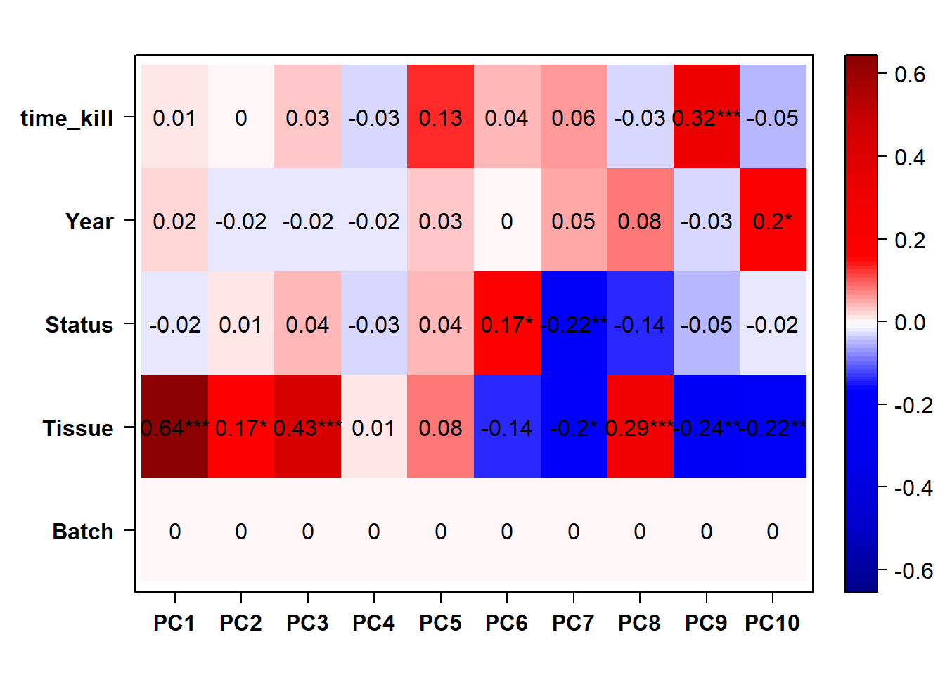
The PCA plot shows that this makes the differences between batches worse apparently stronger, even though the eigencorplot (correlation between PC axis and variable) doesn’t show it. This is probably due to linear combinations of the batch and tissue variables.