Volcano Plots
We do not show the volcano plots here, but they are in the
supplementary material Section 3.
rm(list= ls()[!(ls() %in% keep)])
setwd("../DE_results/")
files<- list.files(pattern="results_[a-zA-Z]+_Status.csv", ignore.case=TRUE)
files<- files[-3]
status_results<- lapply(files, read.csv)
names(status_results)<- word(files, 2, sep="_")
output<- list()
plots<- list()
directionalp<- list()
pos_neg<- list()
for(i in tissue_order){
tissue<- status_results[[i]]
tissue<- tissue[!is.na(tissue$pvalue),]
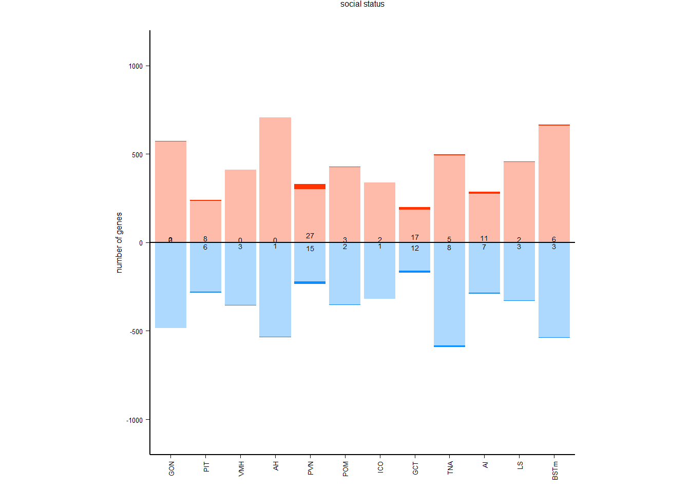
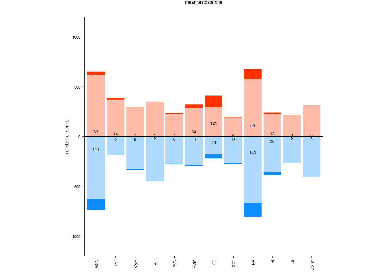
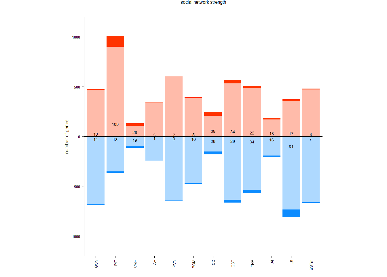
## counts of positive and negative genes
pos_out<- tissue
pos_out$neg_sig<- ifelse(pos_out$padj<0.1 & pos_out$log2FoldChange<0,1,0)
pos_out$neg_marg<- ifelse(pos_out$pvalue<0.05 & pos_out$padj>0.1 & pos_out$log2FoldChange<0,1,0)
pos_out$pos_sig<- ifelse(pos_out$padj<0.1 & pos_out$log2FoldChange>0,1,0)
pos_out$pos_marg<- ifelse(pos_out$pvalue<0.05 & pos_out$padj>0.1 & pos_out$log2FoldChange>0,1,0)
pos_neg[[i]]<- data.frame(tissue=i, res=c(-sum(pos_out$neg_sig, na.rm=TRUE), -sum(pos_out$neg_marg, na.rm=TRUE), sum(pos_out$pos_sig, na.rm=TRUE), sum(pos_out$pos_marg, na.rm=TRUE)), type=c("negative significant", "negative marginal", "positive significant","positive marginal"))
##plots
tissue$gene<- plyr::revalue(tissue$gene, c("LOC113993669"="CYP19A1","LOC113983511"="OXT", "LOC113983498"="AVP", "LOC113982601"="AVPR2"))
tissue$sig<- ifelse(tissue$padj<0.1,"Q<0.1",ifelse(tissue$pvalue<0.05,"P<0.05","NS"))
tissue<- tissue[order(tissue$padj),]
rownames(tissue)<- 1:nrow(tissue)
#tissue$interesting_genes<- ifelse((tissue$gene %in% candidates & tissue$pvalue<0.05) | rownames(tissue) %in% topgenes, as.character(tissue$gene), "")
#tissue$is_interesting<- tissue$interesting_genes==""
#plots[[i]]<- ggplot(tissue, aes(x=log2FoldChange, y=-log10(padj), color=sig)) + geom_point(size=4) + geom_hline(yintercept=-log10(0.1), linetype="dashed", color = "grey70", size=1) + geom_text_repel(aes(label=interesting_genes), color="grey40",size=8, label.padding=1, force_pull=0, force=6) + peri_theme + geom_point(data=tissue[tissue$interesting_genes!="",], aes(fill=sig), pch=21,color="grey40", show.legend=FALSE, size=5) + scale_color_manual(values=tissue_cols[[i]]) + scale_fill_manual(values=tissue_cols[[i]][2:3]) + labs(title=i,subtitle=paste0(nrow(tissue),"/",nrow(tissue[which(tissue$pvalue<0.05),]),"/",nrow(tissue[which(tissue$padj<0.1),])),x="", y="") + scale_x_continuous(limits=c(-4,4), breaks=c(-4,-3,-2,-1,0,1,2,3,4)) + scale_y_continuous(limits=c(0,5))
tissue$X<- NULL
tissue$pvalue<- ifelse(is.na(tissue$padj), NA, as.numeric(tissue$pvalue))
sub<- subset(tissue, select=c("gene","log2FoldChange","pvalue"))
tissue<- subset(tissue, select=c("gene","pvalue"))
colnames(tissue)[colnames(tissue)=="pvalue"] <- i
output[[i]]<- tissue
sub$logP<- -log(sub$pvalue, 10)
sub$logP<- ifelse(sub$log2FoldChange<0, -(sub$logP), sub$logP)
sub<- subset(sub, select=c("gene", "logP"))
colnames(sub)[colnames(sub)=="logP"] <- i
directionalp[[i]]<- sub
}
setwd("../analysis/")
Pairwise Tissue
Similarities
Pulling out the p-value data.
temp<- merge(output[[1]],output[[2]],by="gene", all=TRUE)
temp<- merge(temp, output[[3]], by="gene", all=TRUE)
temp<- merge(temp, output[[4]], by="gene", all=TRUE)
temp<- merge(temp, output[[5]], by="gene", all=TRUE)
temp<- merge(temp, output[[6]], by="gene", all=TRUE)
temp<- merge(temp, output[[7]], by="gene", all=TRUE)
temp<- merge(temp, output[[8]], by="gene", all=TRUE)
temp<- merge(temp, output[[9]], by="gene", all=TRUE)
temp<- merge(temp, output[[10]], by="gene", all=TRUE)
temp<- merge(temp, output[[11]], by="gene", all=TRUE)
pvalue_data<- merge(temp, output[[12]], by="gene", all=TRUE)
rownames(pvalue_data)<- pvalue_data$gene

pvalue_data$gene<- NULL
and the directional log-transformed p-values:
temp<- merge(directionalp[[1]],directionalp[[2]],by="gene", all=TRUE)
temp<- merge(temp, directionalp[[3]], by="gene", all=TRUE)
temp<- merge(temp, directionalp[[4]], by="gene", all=TRUE)
temp<- merge(temp, directionalp[[5]], by="gene", all=TRUE)
temp<- merge(temp, directionalp[[6]], by="gene", all=TRUE)
temp<- merge(temp, directionalp[[7]], by="gene", all=TRUE)
temp<- merge(temp, directionalp[[8]], by="gene", all=TRUE)
temp<- merge(temp, directionalp[[9]], by="gene", all=TRUE)
temp<- merge(temp, directionalp[[10]], by="gene", all=TRUE)
temp<- merge(temp, directionalp[[11]], by="gene", all=TRUE)
logpvalue_data<- merge(temp, directionalp[[12]], by="gene", all=TRUE)
rownames(logpvalue_data)<- logpvalue_data$gene
logpvalue_data$gene<- NULL
logpvalue_status<- logpvalue_data
keep<- c(keep, "logpvalue_status")
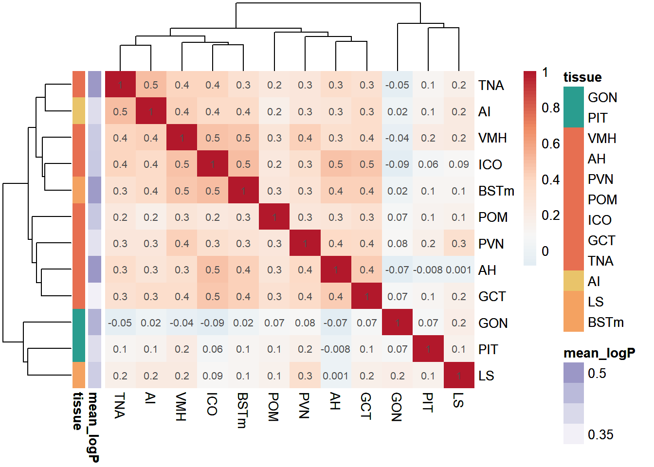
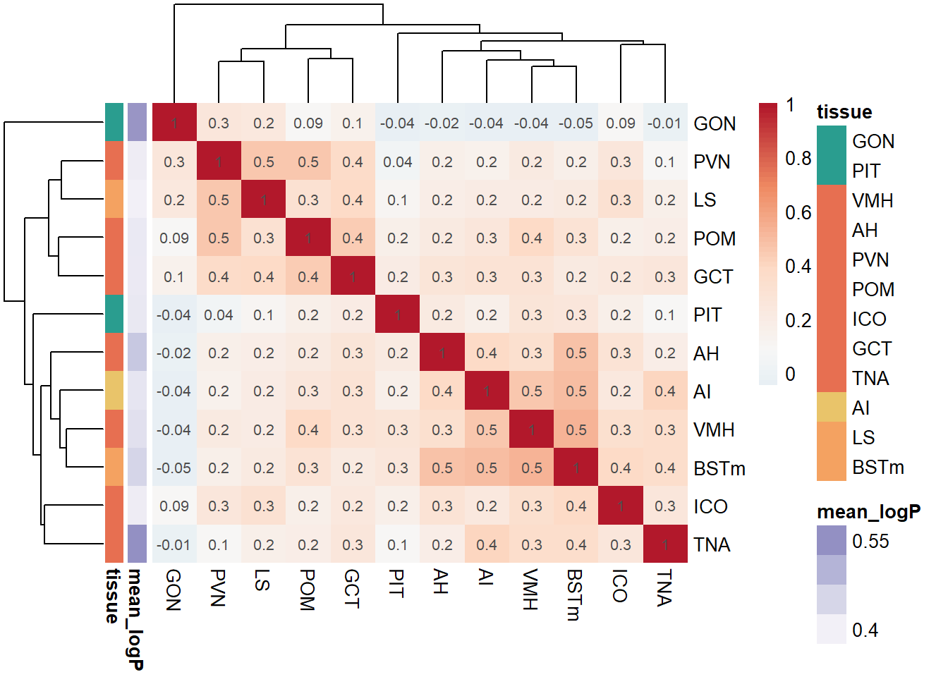
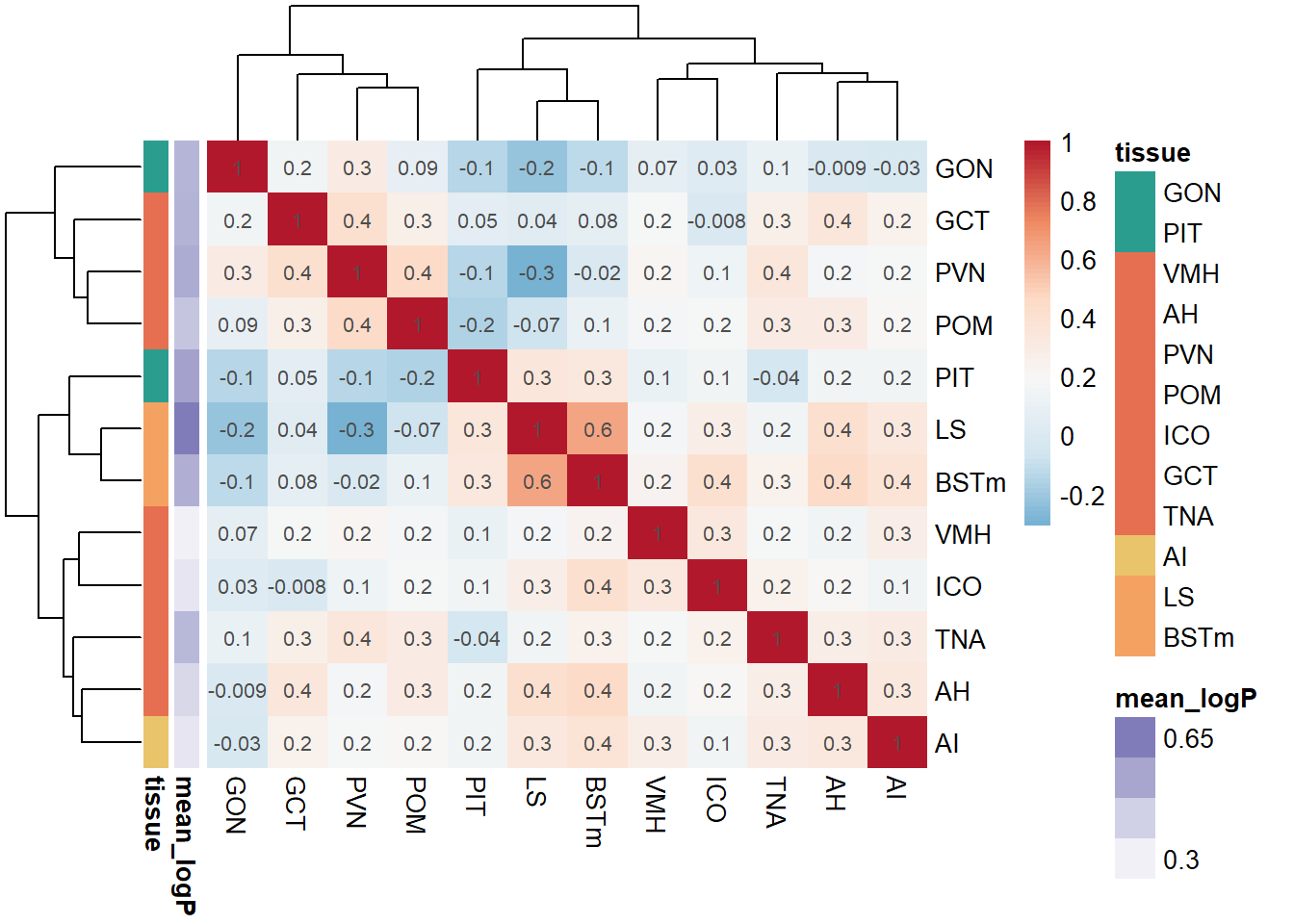
pvalue_cor<- cor(logpvalue_data, use= "pairwise.complete.obs", method="pearson")
xy <- t(combn(colnames(pvalue_cor), 2))
xy<- data.frame(xy, dist=pvalue_cor[xy])
#hist(xy$dist, breaks=20)
#min(xy$dist)
mean(xy$dist)
FALSE [1] 0.2349926
ps<-colorRampPalette(brewer.pal(n = 7, name =
  "Purples"))(100)

#color=colorRampPalette(brewer.pal(n = 7, name ="YlOrRd"))(100)
color=rev(colorRampPalette(brewer.pal(n = 7, name =
  "RdBu"))(100))


exp<- data.frame(row.names=colnames(logpvalue_data),mean_logP=apply(-log10(pvalue_data),2, mean,na.rm=TRUE)) #using the raw p-value data here because taking the average of directional p-values would be silly.
exp$tissue<- tissue_order
ann_cols<- list(tissue=tissue_colors, mean_logP=ps[1:52]) #Max mean_log pvalue is 0.52


p<- pheatmap(pvalue_cor, color=color[42:100], annotation_row=exp, border_color = NA, display_numbers = signif(pvalue_cor,1), annotation_colors = ann_cols, clustering_distance_cols = "euclidean", clustering_distance_rows = "euclidean", clustering_method="complete")
p
save_pheatmap_png(p, filename="../Overlap_results/heatmap_status", width=800, height=800)
FALSE png
FALSE   2
xy_status<-
ggplot(xy, aes(x=dist, fill=..x..)) + geom_histogram(color="grey80", size=0.3) + scale_fill_gradient2(low=color[42], high = color[74]) + peri_figure + scale_y_continuous(expand=c(0,0), limits=c(0,15)) + theme(legend.position="none", aspect.ratio = 0.2) + labs(x="r") + scale_x_continuous(limits=c(-1,1)) + geom_vline(aes(xintercept=mean(dist)),
color="grey70", linetype="dashed", size=0.3)
keep<- c(keep, "xy_status")
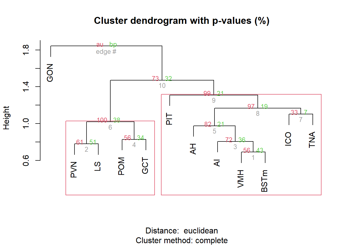
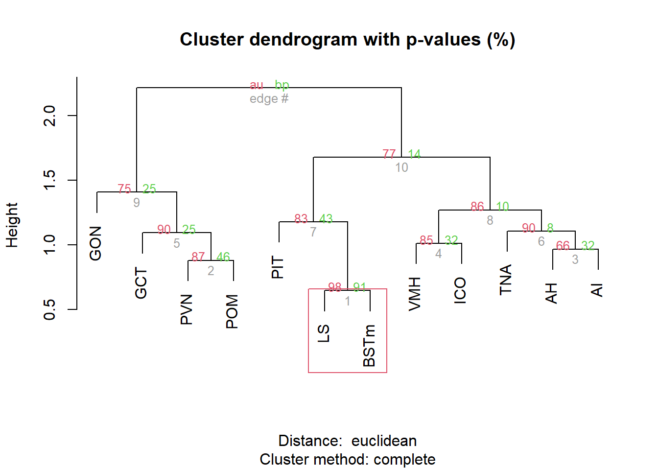
result <- pvclust(pvalue_cor, method.dist="euclidean", method.hclust="complete", nboot=10000, parallel=TRUE)
FALSE Creating a temporary cluster...done:
FALSE socket cluster with 7 nodes on host 'localhost'
FALSE Multiscale bootstrap... Done.
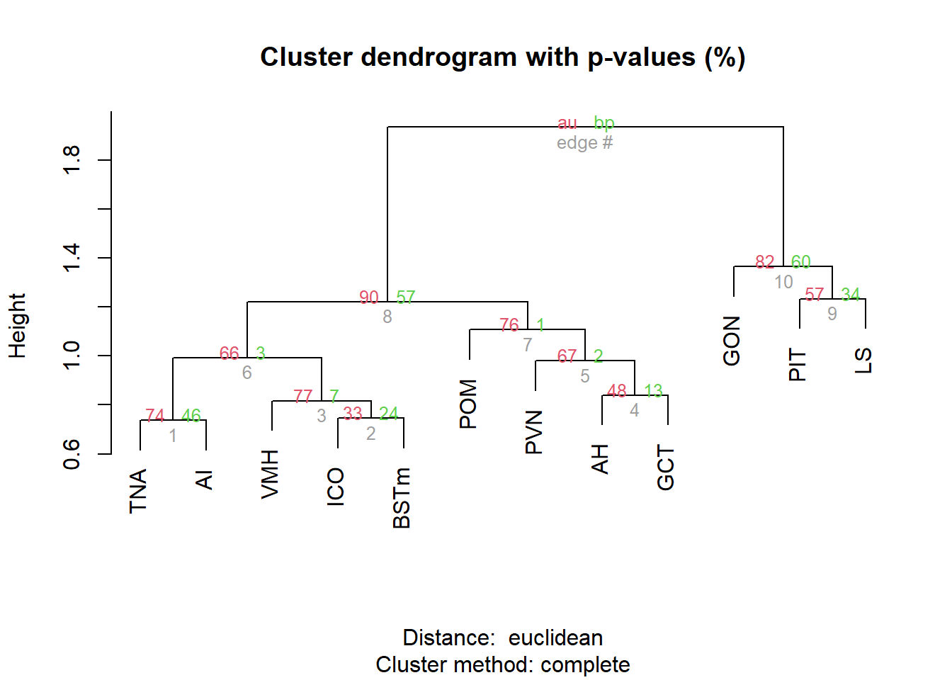
pvrect(result, alpha=0.90)
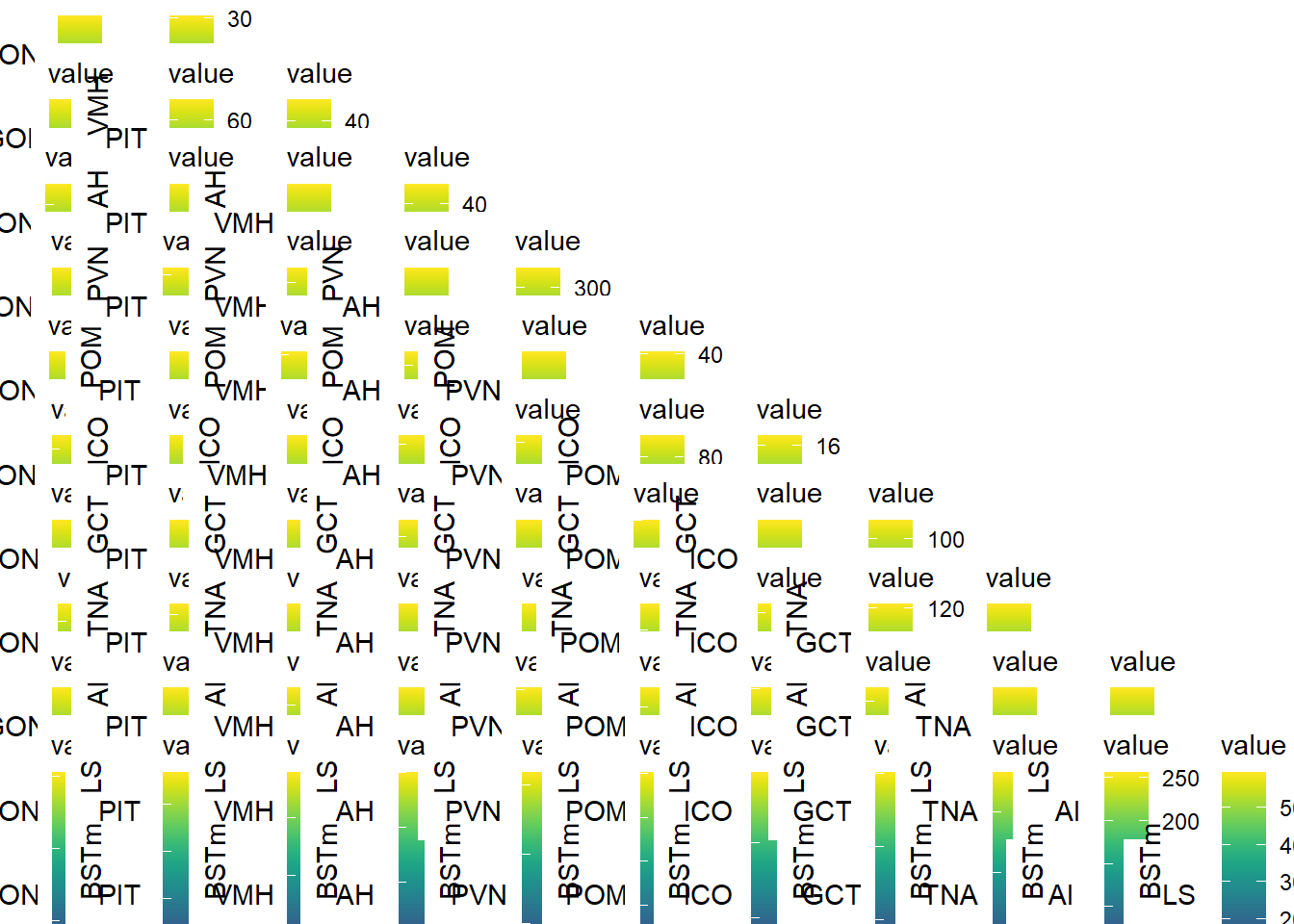
RRHO2
This approach uses package ‘RRHO2’ and compares rank ordered gene
lists against each-other and uses a hypergeometric test to compare the
similarity of gene names in shorter segments along the length gene
list.
The results reported in the paper are scaled to the largest log10
P-value in all of the pairwise comparisons, as a visual aid to help
scale for multiple comparisons across tissues. However, we also present
the unscaled versions too.
RRHO_objects<- list()

comparisons<- combn(tissue_order, 2)
RRHO_objects<- list()
for(i in 1:ncol(comparisons)){
  comparison<- comparisons[,i]
  p1_name<- comparison[1]
  p2_name<- comparison[2]
  p1<- data.frame(gene=row.names(logpvalue_data), logP_1=logpvalue_data[,p1_name])
  p2<- data.frame(gene=row.names(logpvalue_data), logP_2=logpvalue_data[,p2_name])
  comb<- merge(p1,p2)
  comb<- comb[complete.cases(comb),]
  p11<- comb[, c("gene","logP_1")]
  p11<- p11[order(p11$logP_1, decreasing=TRUE),]
  p22<- comb[,c("gene","logP_2")]
  p22<- p22[order(p22$logP_2, decreasing=TRUE),]
  p1_p2<- paste(p1_name,p2_name, sep="_")
  RRHO_objects[[p1_p2]]<- RRHO2_initialize(p11, p22, labels = c(p1_name, p2_name), log10.ind=TRUE, boundary=0.01)
  #jpeg(filename=paste0("RRHO2_status",p1_p2,".jpg"))
  #RRHO2_heatmap(RRHO_objects[[p1_p2]])
  #dev.off()
}
save(RRHO_objects,file="../Overlap_results/RRHO2/RRHO2_Status.RData")
#load("../Overlap_results/RRHO2/RRHO2_Status.RData")


maxp<- vector(mode="numeric")
for(i in names(RRHO_objects)){
  sub<- RRHO_objects[[i]]$hypermat
  maxp[i]<- max(sub, na.rm=TRUE)
}
maxp<- max(maxp)

plots_scaled<- list() # for the plots on the same scale
plots<- list()
for(i in names(RRHO_objects)){
  sub<- RRHO_objects[[i]]$hypermat
  sub<- melt(sub, na.rm=TRUE)
  x<- word(i,1,1,sep="_")
  y<- word(i,2,2,sep="_")
  plots_scaled[[i]]<- ggplot(data=sub, aes(Var1, Var2, fill=value)) + geom_tile() + peri_theme + scale_y_continuous(expand=c(0,0)) + scale_x_continuous(expand=c(0,0)) + scale_fill_viridis(limits=c(0,maxp)) + theme(axis.text.x=element_blank(),axis.text.y=element_blank(), axis.ticks=element_blank(), legend.position="none") + labs(x=x, y=y)
  plots[[i]]<- ggplot(data=sub, aes(Var1, Var2, fill=value)) + geom_tile() + scale_y_continuous(expand=c(0,0)) + scale_x_continuous(expand=c(0,0)) + scale_fill_viridis() + theme(axis.text.x=element_blank(),axis.text.y=element_blank(), axis.ticks=element_blank()) + labs(x=x, y=y)
}


m <- matrix(NA, 11, 11)
m[lower.tri(m, diag = T)] <- 1:66

## This plot is just to farm the legend.
p<- ggplot(data=sub, aes(Var1, Var2, fill=value)) + geom_tile() + peri_theme + scale_y_continuous(expand=c(0,0)) + scale_x_continuous(expand=c(0,0)) + scale_fill_viridis(limits=c(0,maxp)) + theme(axis.text.x=element_blank(),axis.text.y=element_blank(), axis.ticks=element_blank()) + labs(x=x, y=y)
leg<- get_legend(p)

m1<- m
m1[1,11]<- 67
plots_scaled[["legend"]]<- leg
g<-arrangeGrob(grobs= plots_scaled, layout_matrix = m1)

ggsave(file="../Overlap_results/RRHO2/figure_RRHO_status_scaled.pdf", g, units="in", width=20, height=20)


g<-grid.arrange(grobs= plots, layout_matrix = m)
ggsave(file="../Overlap_results/RRHO2/figure_RRHO_status_unscaled.pdf", g, units="in", width=25, height=15)
I don’t know how to get these figures to not look crappy on the
markdown so they are available to view as a raw pdf. The scaled PDF is
HERE,
and the unscaled is HERE.
Overall brain
patterns
Here I am taking just the brain tissues and taking the median p-value
of each gene in the rank-ordered gene list. This will give an idea for
similar gene expression patterns across the entire brain.
brain<- logpvalue_data[,-c(1:2)]
brain$p_combo<- apply(brain,1, median)
brain<- brain[complete.cases(brain),]
brain$gene<- rownames(brain)
brain_go<- merge(brain, go_terms, by="gene", all.x=TRUE)
brain_go<- brain_go[order(brain_go$p_combo, decreasing=TRUE),]
write.csv(brain,"../Overlap_results/results_brain_status.csv", row.names=FALSE)
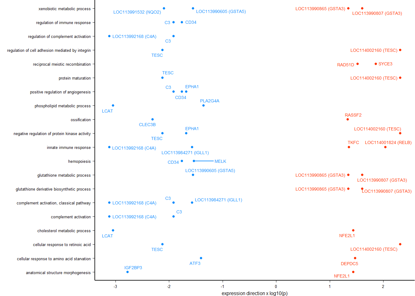
geneList<- brain_go$p_combo
names(geneList)<- brain_go$gene
#subsets<- brain[brain$p_combo>=1.3,]
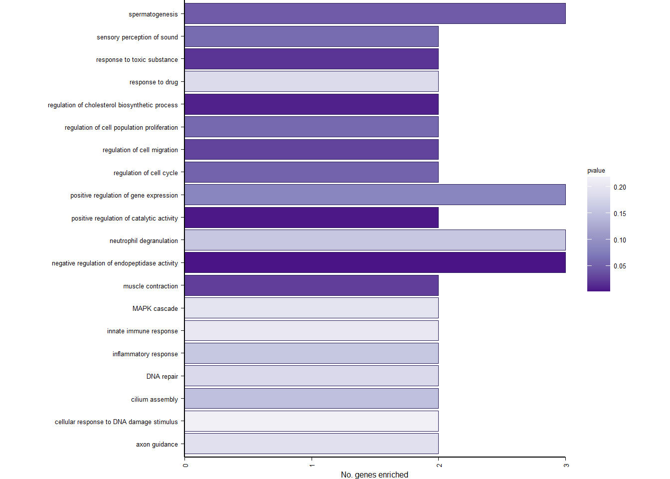
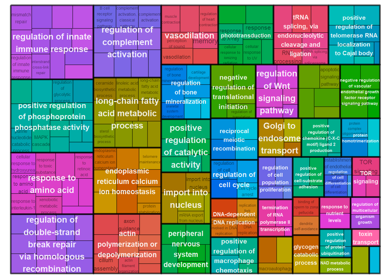
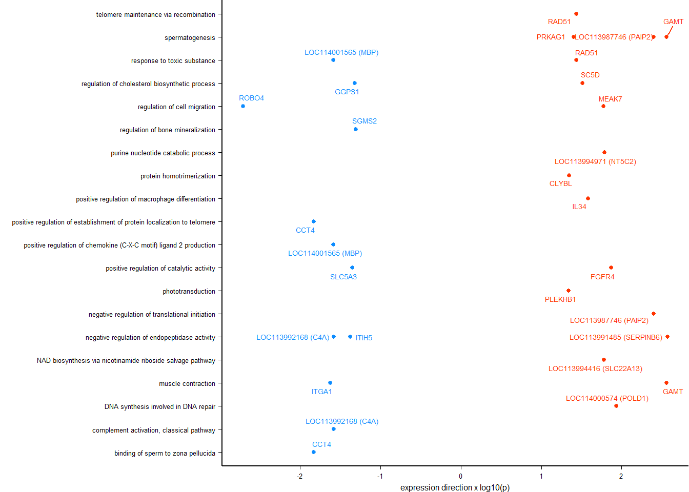
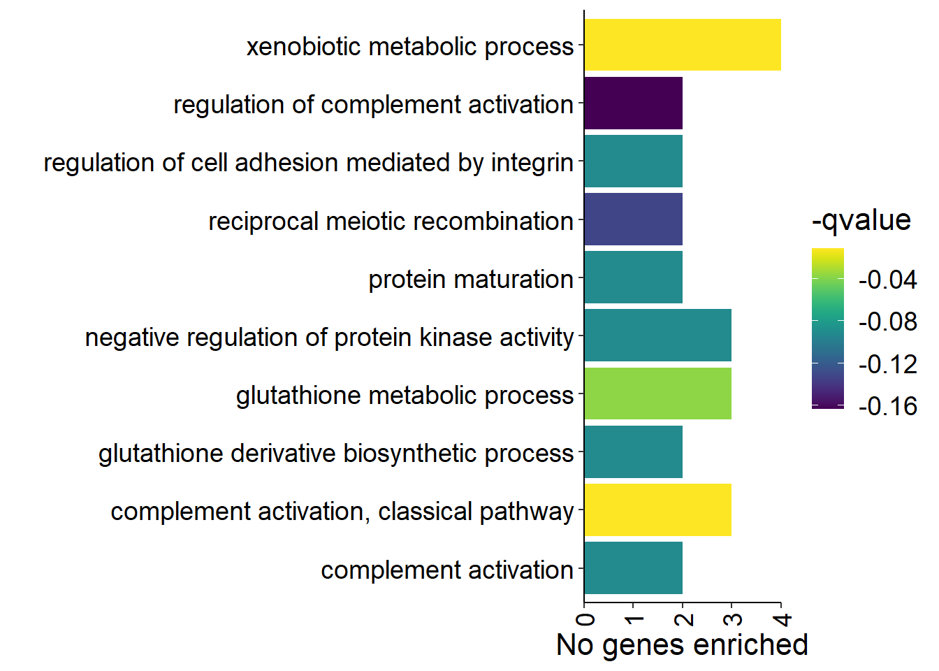
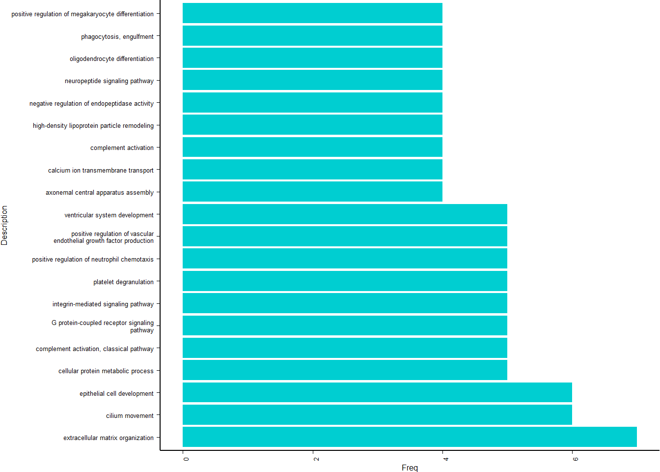
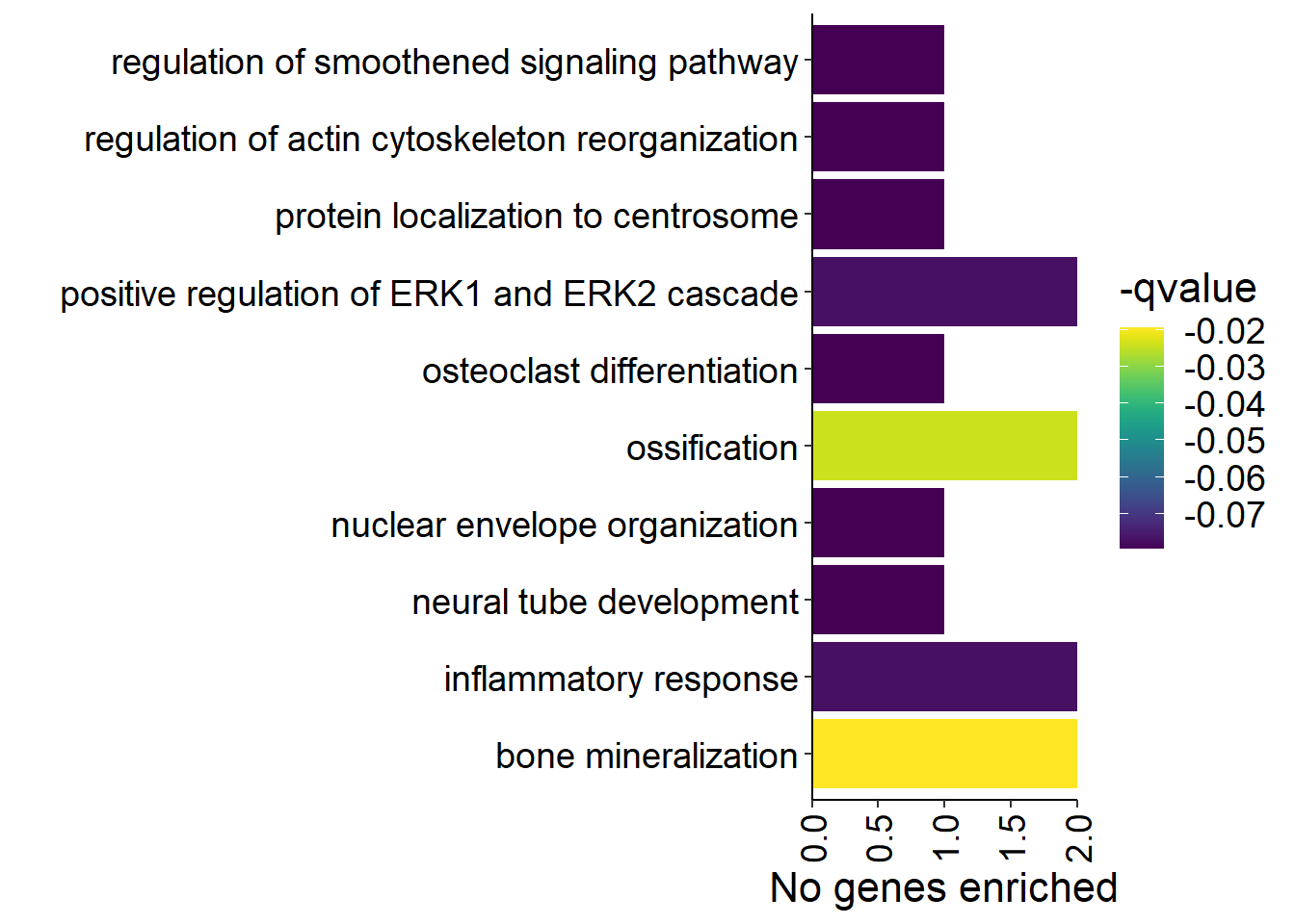
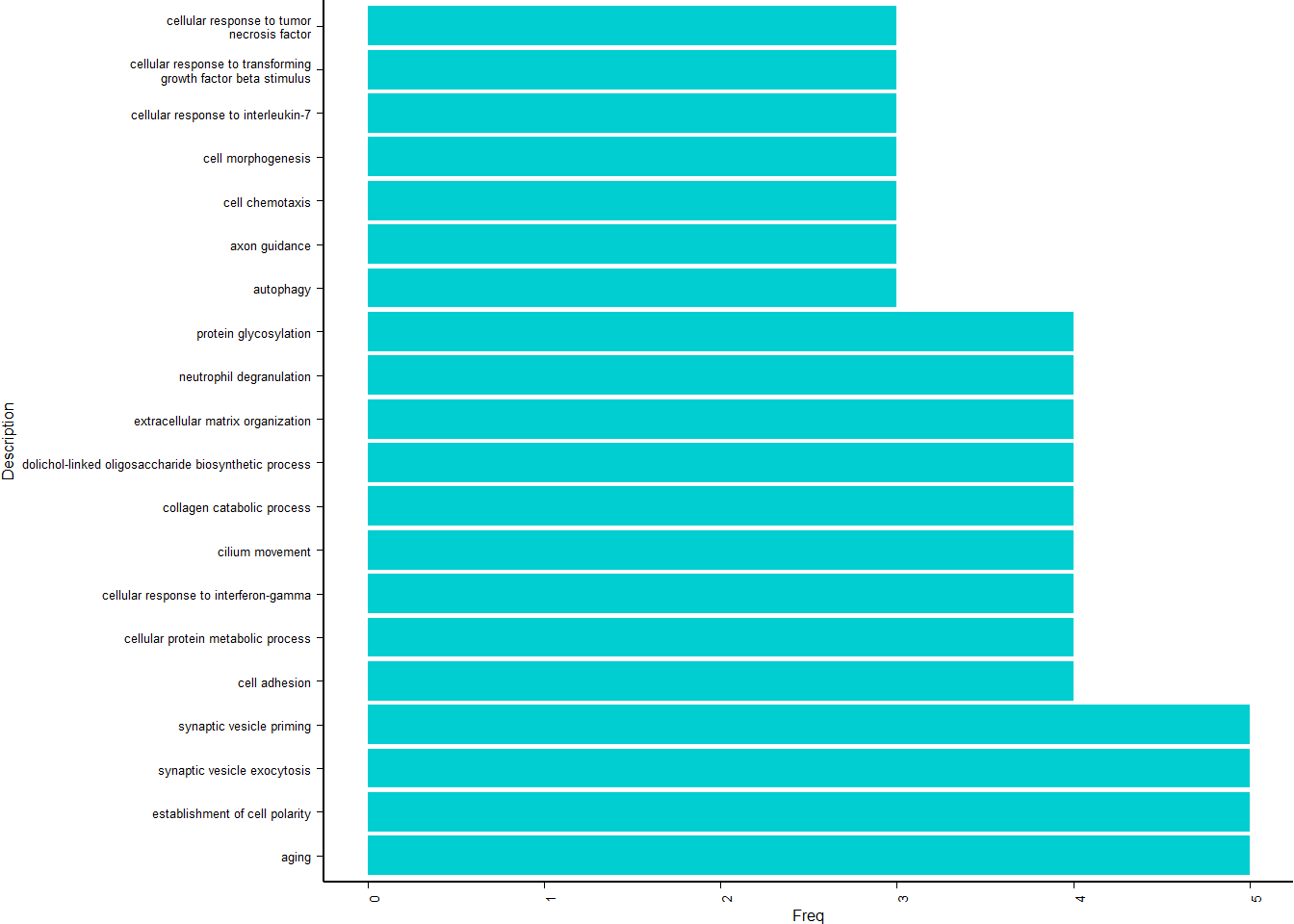
y<- enricher(brain$gene[which(abs(brain$p_combo)>1.3)], universe=brain$gene, TERM2GENE = go2gene_bp, TERM2NAME = go2name_bp)
#ridgeplot(y)
ego2<- y@result
ego2$GeneRatio2<- word(ego2$GeneRatio, 1,1, sep="/")
ego2$GeneRatio2<- as.numeric(ego2$GeneRatio2)
ego2<- ego2[ego2$GeneRatio2>1,]
p<- ggplot(ego2[1:20,], aes(x=Description, y=GeneRatio2, fill=pvalue)) + geom_bar(stat="identity", size=0.3, color="#2A1E59") + theme(axis.text.x=element_text(angle=90, vjust=0.5, hjust=1.2)) + coord_flip() + peri_figure + scale_y_continuous(expand=c(0,0)) + labs(x="", y="No. genes enriched") + theme(aspect.ratio = 1.2) + scale_fill_distiller(palette="Purples")
p
ggsave("../Overlap_results/figure_brain_GO_status.pdf", plot=p, device="pdf", height=1.60, width=4.60, units="in")


knitr::kable(y@result[1:10,], caption="BP enriched GO terms in the median p in the brain", row.names = FALSE) %>% kable_styling()
BP enriched GO terms in the median p in the brain
|
ID
|
Description
|
GeneRatio
|
BgRatio
|
pvalue
|
p.adjust
|
qvalue
|
geneID
|
Count
|
|
GO:0010951
|
negative regulation of endopeptidase activity
|
3/45
|
59/11064
|
0.0017434
|
0.2521041
|
0.2362749
|
ITIH5/LOC113991485/LOC113992168
|
3
|
|
GO:0043085
|
positive regulation of catalytic activity
|
2/45
|
22/11064
|
0.0035482
|
0.2521041
|
0.2362749
|
FGFR4/SLC5A3
|
2
|
|
GO:0045540
|
regulation of cholesterol biosynthetic process
|
2/45
|
33/11064
|
0.0078834
|
0.2521041
|
0.2362749
|
GGPS1/SC5D
|
2
|
|
GO:0009636
|
response to toxic substance
|
2/45
|
54/11064
|
0.0202447
|
0.2521041
|
0.2362749
|
LOC114001565/RAD51
|
2
|
|
GO:0006936
|
muscle contraction
|
2/45
|
61/11064
|
0.0254302
|
0.2521041
|
0.2362749
|
GAMT/ITGA1
|
2
|
|
GO:0030334
|
regulation of cell migration
|
2/45
|
66/11064
|
0.0294294
|
0.2521041
|
0.2362749
|
MEAK7/ROBO4
|
2
|
|
GO:0000731
|
DNA synthesis involved in DNA repair
|
1/45
|
10/11064
|
0.0399520
|
0.2521041
|
0.2362749
|
LOC114000574
|
1
|
|
GO:0007602
|
phototransduction
|
1/45
|
10/11064
|
0.0399520
|
0.2521041
|
0.2362749
|
PLEKHB1
|
1
|
|
GO:0034356
|
NAD biosynthesis via nicotinamide riboside salvage pathway
|
1/45
|
10/11064
|
0.0399520
|
0.2521041
|
0.2362749
|
LOC113994416
|
1
|
|
GO:0045651
|
positive regulation of macrophage differentiation
|
1/45
|
10/11064
|
0.0399520
|
0.2521041
|
0.2362749
|
IL34
|
1
|
write.csv(y@result,"../Overlap_results/GO_status_brain.csv", row.names=FALSE)
#y<- GSEA(geneList, TERM2GENE = go2gene_bp, TERM2NAME = go2name_bp)
#ridgeplot(y)
#write.csv(y@result,"GSEA_status_brain.csv", row.names=FALSE)
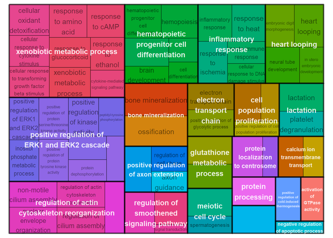
ego2<- as.data.frame(y@result$ID)
colnames(ego2)<- "ID"
ego2$p.adjust<- y@result$p.adjust
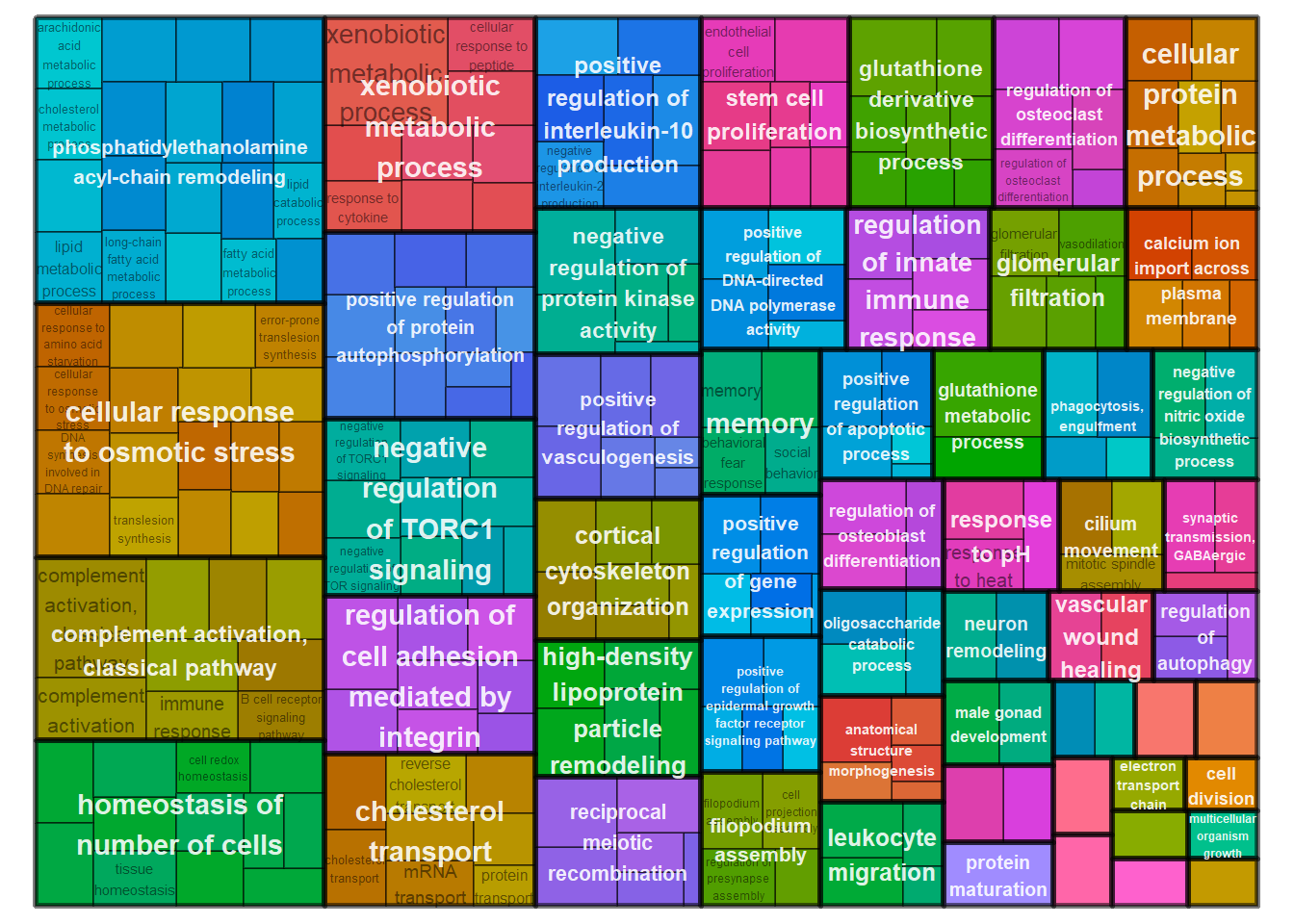
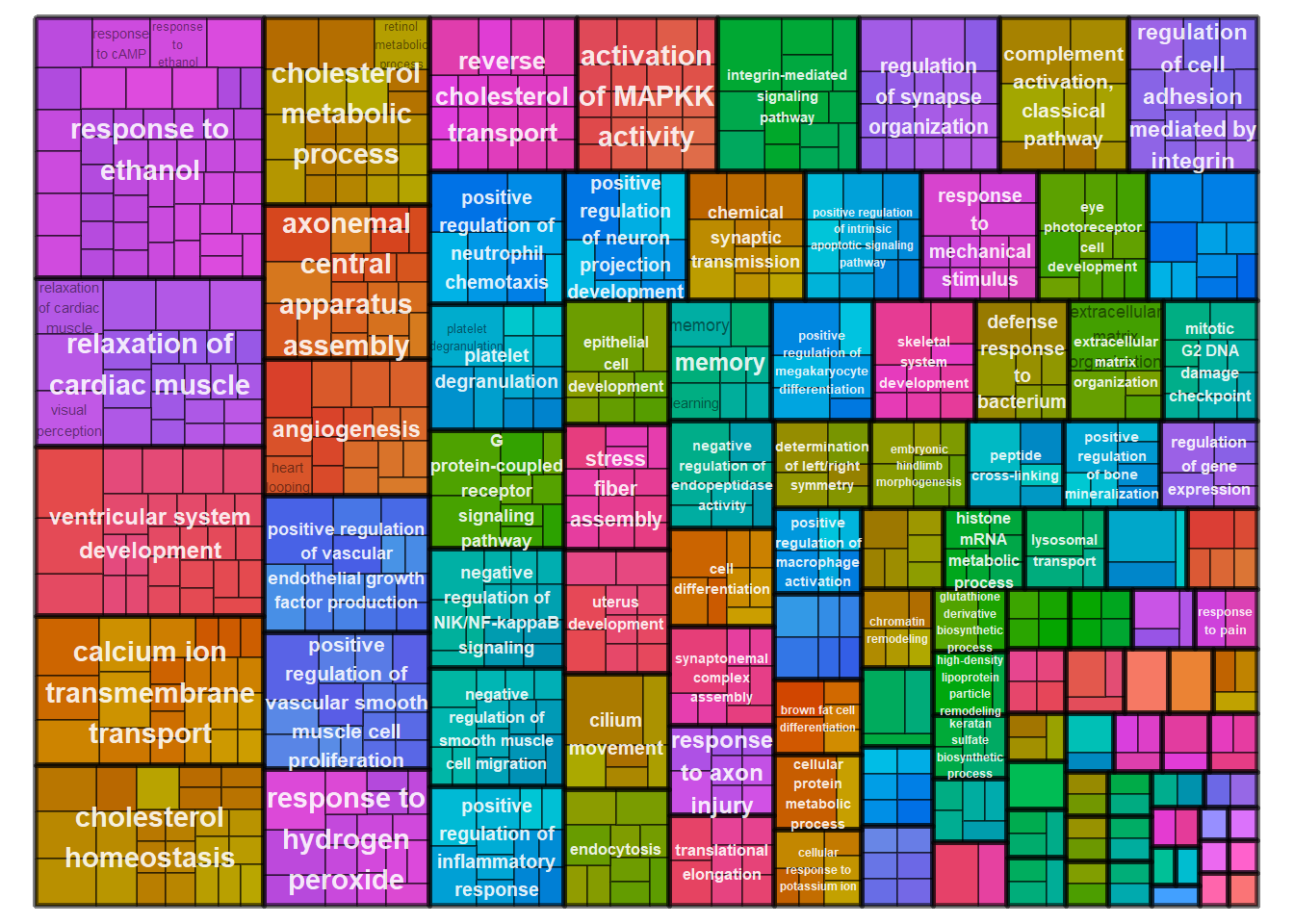
simMatrix <- calculateSimMatrix(ego2$ID,
orgdb="org.Hs.eg.db",
ont="BP",
method="Rel")
scores <- setNames(-log10(ego2$p.adjust), ego2$ID)
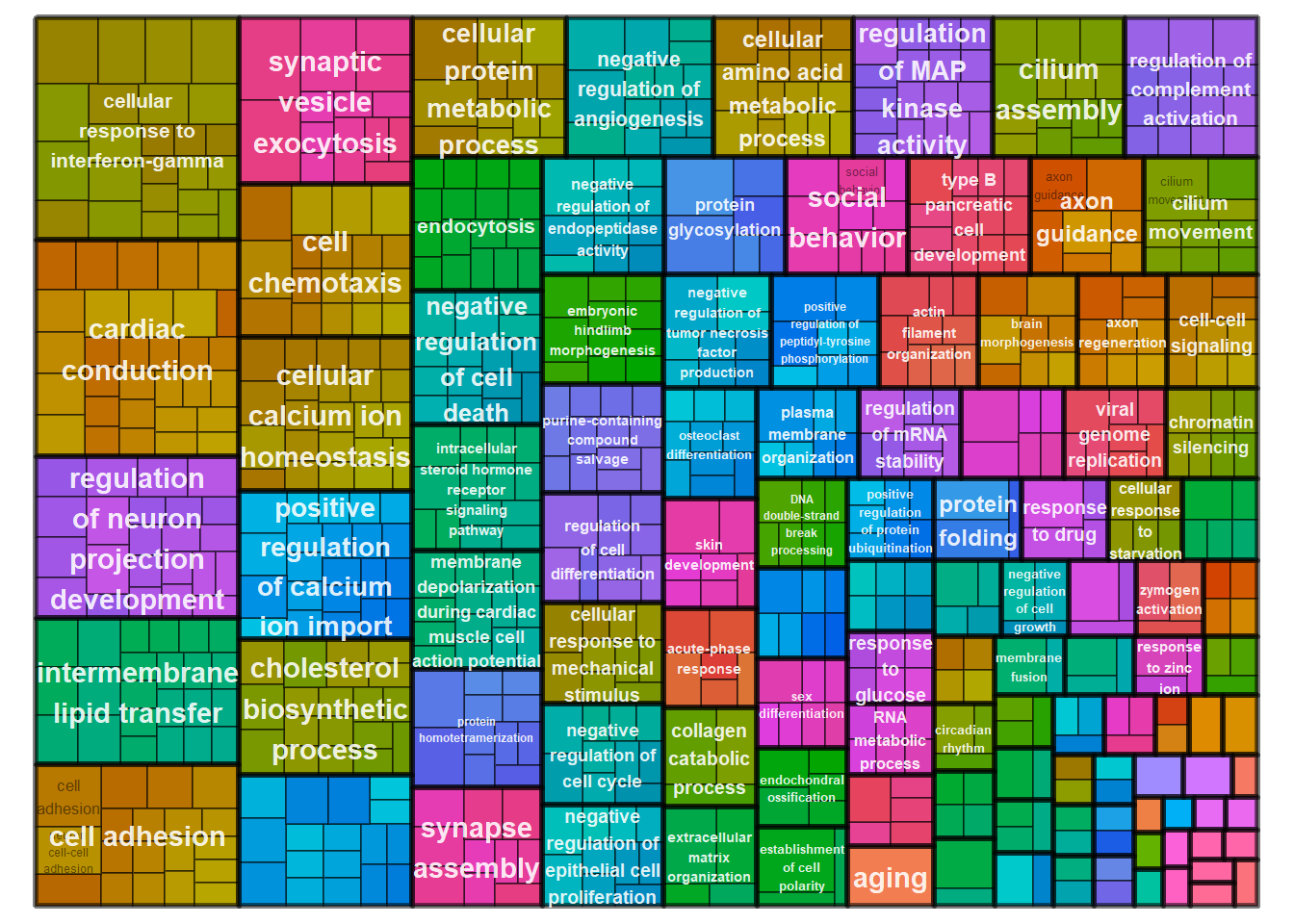
reducedTerms <- reduceSimMatrix(simMatrix,
scores,
threshold=0.7,
orgdb="org.Hs.eg.db")
treemapPlot(reducedTerms)
#heatmapPlot(simMatrix,
#            reducedTerms,
#            annotateParent=TRUE,
#            annotationLabel="parentTerm",
#            fontsize=6)
tophits<- brain
tophits$p_combo<- abs(tophits$p_combo)
tophits<- tophits[order(tophits$p_combo, decreasing=TRUE),]
tophits<- tophits$gene[1:10]
out<- list()
#i="POM"
for(i in tissue_order){
tissue<- status_results[[i]]
tissue<- tissue[!is.na(tissue$pvalue),]
sub<- tissue[tissue$gene %in% tophits,]
out[[i]]<- data.frame(gene=sub$gene, lfc=sub$log2FoldChange, p=sub$pvalue, padj=sub$padj, Tissue=i)
}
status_results_tophits<- do.call("rbind", out)
status_results_tophits<- status_results_tophits[status_results_tophits$Tissue!="GON" & status_results_tophits$Tissue!="PIT",]
outliers=c("PFT2_POM_run1")
brain_behav<- subset(key_behav, Tissue!="GON")
brain_behav<- subset(brain_behav, Tissue!="PIT")
brain_behav<- brain_behav[!rownames(brain_behav) %in% outliers,]
brain_behav<- droplevels(brain_behav)
brain_data<- data[,colnames(data) %in% rownames(brain_behav)]
start<- nrow(brain_data)
#remove genes with avg read counts <20
brain_data$avg_count<- apply(brain_data, 1, mean)
brain_data<- brain_data[brain_data$avg_count>20,]
brain_data$avg_count<-NULL
#remove genes where >50% of samples have 0 gene expression
brain_data$percent_0<- apply(brain_data, 1, function(x)length(x[x==0]))
thresh<- ncol(brain_data)/2
brain_data<- brain_data[brain_data$percent_0<=thresh,]
brain_data$percent_0<-NULL
#13652 genes.
dd<- DESeqDataSetFromMatrix(countData=brain_data, colData=brain_behav, design= ~ Tissue + Status)
dd<- DESeq(dd)
dd<- dd[which(mcols(dd)$betaConv),] #remove any genes that didn't converge.
res<- results(dd, alpha=0.1)
gone<- plotCounts(dd, gene=row.names(res[tophits[1],]), intgroup=c("Tissue","Status"), returnData=TRUE)
gtwo<- plotCounts(dd, gene=row.names(res[tophits[2],]), intgroup=c("Tissue","Status"), returnData=TRUE)
gthree<- plotCounts(dd, gene=row.names(res[tophits[3],]), intgroup=c("Tissue","Status"), returnData=TRUE)
gfour<- plotCounts(dd, gene=row.names(res[tophits[4],]), intgroup=c("Tissue","Status"), returnData=TRUE)
gfive<- plotCounts(dd, gene=row.names(res[tophits[5],]), intgroup=c("Tissue","Status"), returnData=TRUE)
gsix<- plotCounts(dd, gene=row.names(res[tophits[6],]), intgroup=c("Tissue","Status"), returnData=TRUE)
vars<- list(gone,gtwo,gthree,gfour,gfive,gsix)
#
plots<- list()
#i=2
for(i in 1:6){
dat<- vars[[i]]
name<- tophits[i]
result<- status_results_tophits[status_results_tophits$gene==name,]
result$label<- paste0("LFC=",signif(result$lfc,2), "\np(raw)=", formatC(result$p,2,format="e"))
result$x<- 1.5
result$y<- max(dat$count)-30
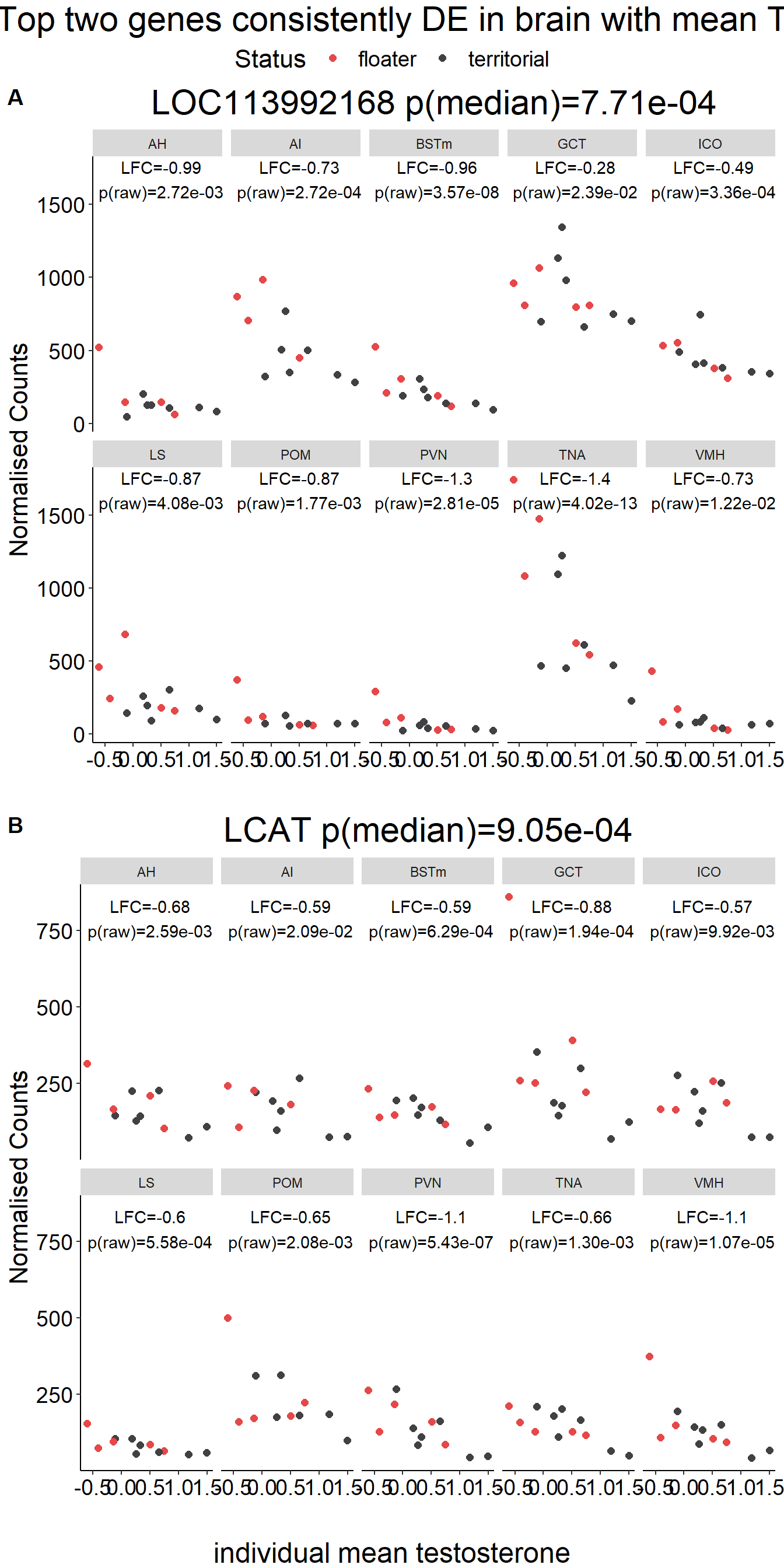
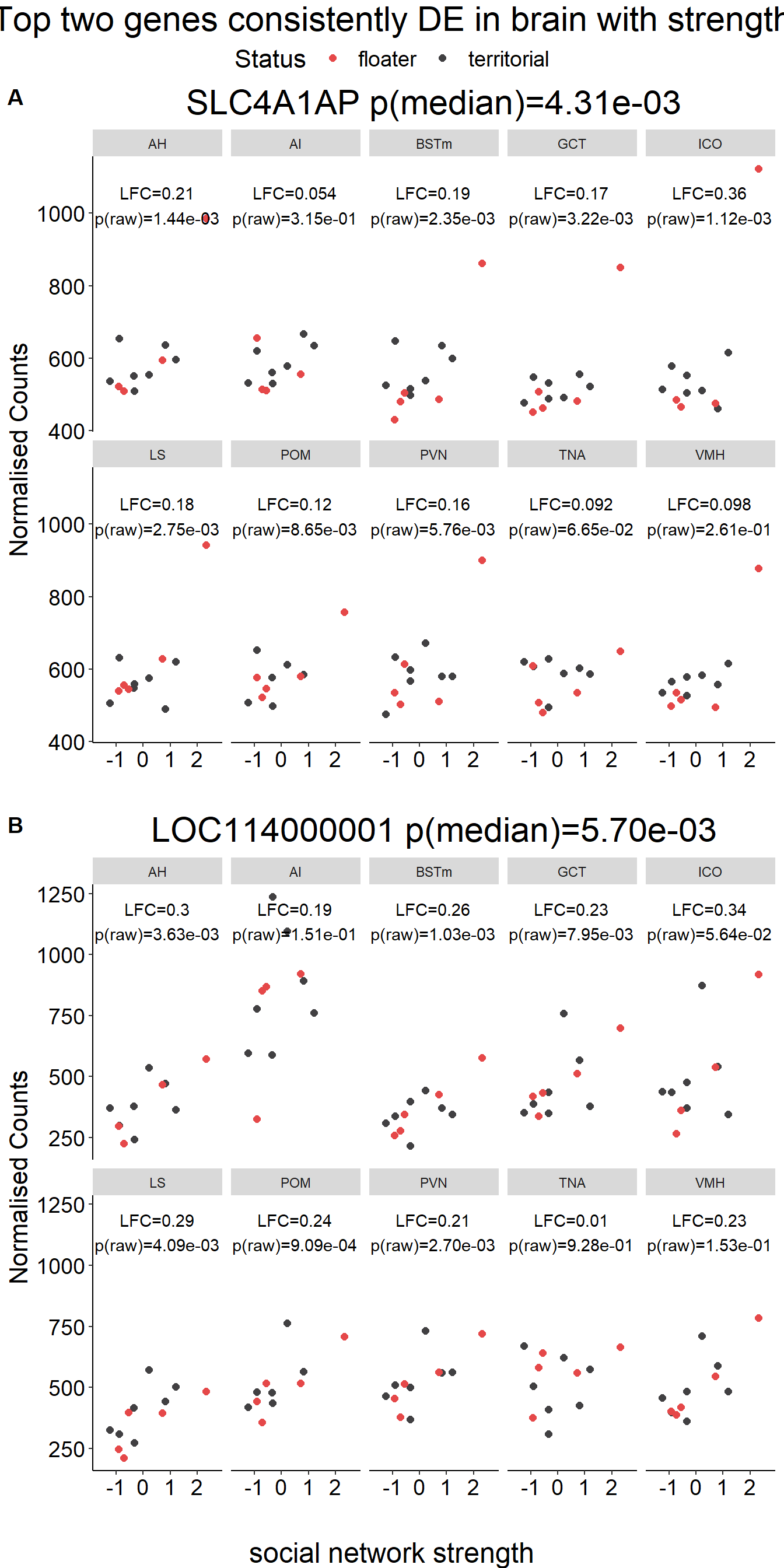
plots[[i]]<- ggplot(dat, aes(x=Status, y=count)) + geom_point(size=2, position=dodge, aes(color=Status)) + geom_boxplot(fill=NA, position=dodge, aes(color=Status)) + labs(title=paste0(name, " p(median)=", formatC(10^-abs(brain_go$p_combo[brain_go$gene==name]),2, format="e")),x="", y="Normalised Counts") + peri_theme + scale_colour_manual(values=status_cols[2:3]) + facet_wrap(. ~Tissue, ncol=5) + geom_text(data=result, aes(x=x, y=y, label=label))
}
g<- ggarrange(plotlist=plots[1:2],ncol=1, nrow=2, common.legend = TRUE, labels=c("A","B"))
g<- annotate_figure(g, top=textGrob("Top two genes consistently DE in brain with social status",gp=gpar(fontsize=22)), bottom=textGrob("social status",gp=gpar(fontsize=18)))
g
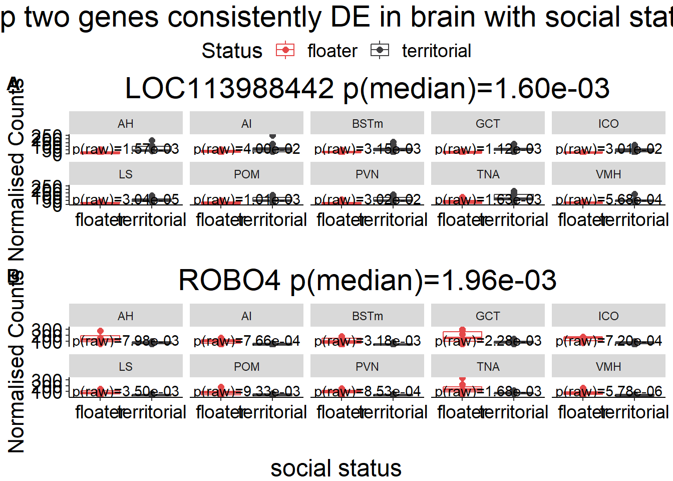
ggexport(g, filename = "../Overlap_results/figure_braintop_status.png", width = 700,height = 900)
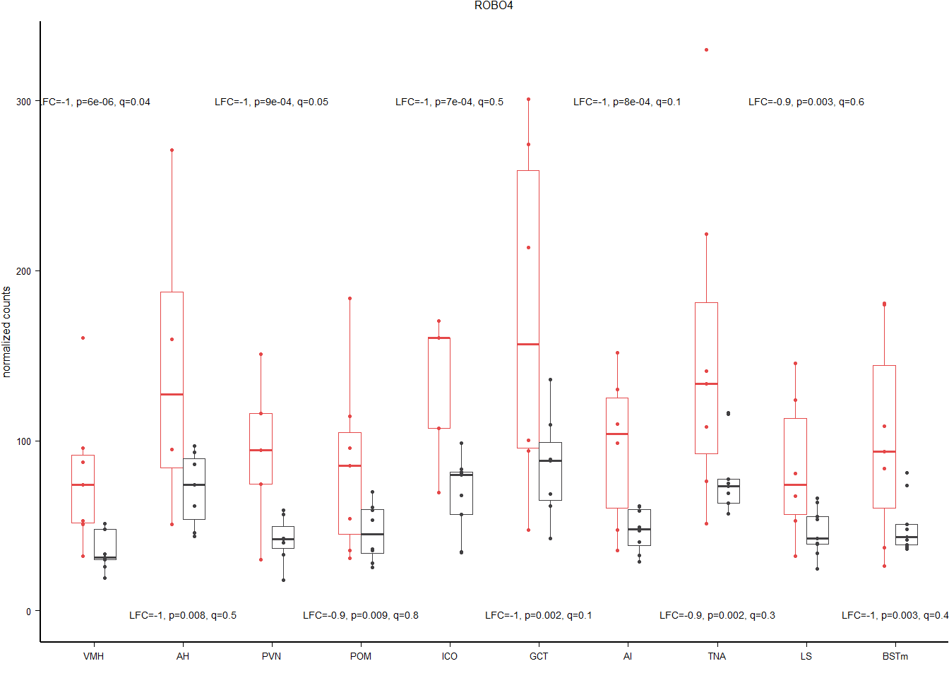
hub=rownames(res[tophits[1],])
gone$Tissue<- factor(gone$Tissue, levels=c("VMH","AH","PVN","POM","ICO","GCT","AI","TNA","LS", "BSTm"))
result<- status_results_tophits[status_results_tophits$gene==hub,]
result$Tissue<- factor(result$Tissue, levels=c("VMH","AH","PVN","POM","ICO","GCT","AI","TNA","LS", "BSTm"))
result<- result[order(result$Tissue),]
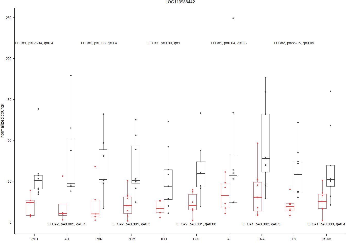
result$label<- paste0("LFC=",signif(result$lfc,1), ", p=", signif(result$p,1), ", q=", signif(result$padj,1))
result$x<- 1.5
result$y<- rep(c(max(gone$count)-30,-2),5)
geom_text.size = (5/14)*(5)
a<- ggplot(gone, aes(x=Tissue, y=count)) + geom_point(size=0.6, pch=19, aes(color=Status), position=position_dodge(0.5)) + geom_boxplot(outlier.shape = NA, fill=NA, aes(color=Status),lwd=0.3, width=0.5, position=position_dodge(0.5)) + peri_figure + scale_colour_manual(values=status_cols[2:3]) + labs(x="", y="normalized counts", title=hub) + theme(legend.position = "none", strip.text = element_text(size=5)) + geom_text(data=result, aes(x=Tissue, y=y, label=label), size=geom_text.size)
a
hub=rownames(res[tophits[2],])
gtwo$Tissue<- factor(gtwo$Tissue, levels=c("VMH","AH","PVN","POM","ICO","GCT","AI","TNA","LS", "BSTm"))
result<- status_results_tophits[status_results_tophits$gene==hub,]

result$Tissue<- factor(result$Tissue, levels=c("VMH","AH","PVN","POM","ICO","GCT","AI","TNA","LS", "BSTm"))
result<- result[order(result$Tissue),]
result$label<- paste0("LFC=",signif(result$lfc,1), ", p=", signif(result$p,1), ", q=", signif(result$padj,1))
result$x<- 1.50
result$y<- rep(c(max(gtwo$count)-30,-2),5)
geom_text.size = (5/14)*(5)
b<- ggplot(gtwo, aes(x=Tissue, y=count)) + geom_point(size=0.6, pch=19, aes(color=Status), position=position_dodge(0.5)) + geom_boxplot(outlier.shape = NA, fill=NA, aes(color=Status),lwd=0.3, width=0.5, position=position_dodge(0.5)) + peri_figure + scale_colour_manual(values=status_cols[2:3]) + labs(x="", y="normalized counts", title=hub) + theme(legend.position = "none", strip.text = element_text(size=5)) + geom_text(data=result, aes(x=Tissue, y=y, label=label), size=geom_text.size)
b
p<- ggarrange(a,b, nrow=2)

ggsave("../Overlap_results/figure_braintop_status.pdf", plot=p, device="pdf", height=3, width=5.5, units="in")
1 Social Status
1.1 Volcano Plots
We do not show the volcano plots here, but they are in the supplementary material Section 3.
1.2 Pairwise Tissue Similarities
Pulling out the p-value data.
and the directional log-transformed p-values:
1.3 RRHO2
This approach uses package ‘RRHO2’ and compares rank ordered gene lists against each-other and uses a hypergeometric test to compare the similarity of gene names in shorter segments along the length gene list.
The results reported in the paper are scaled to the largest log10 P-value in all of the pairwise comparisons, as a visual aid to help scale for multiple comparisons across tissues. However, we also present the unscaled versions too.
I don’t know how to get these figures to not look crappy on the markdown so they are available to view as a raw pdf. The scaled PDF is HERE, and the unscaled is HERE.
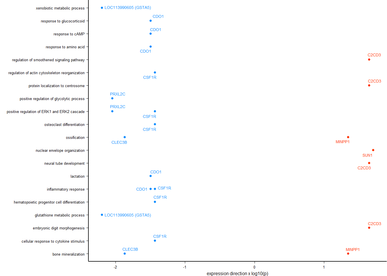
1.4 Overall brain patterns
Here I am taking just the brain tissues and taking the median p-value of each gene in the rank-ordered gene list. This will give an idea for similar gene expression patterns across the entire brain.
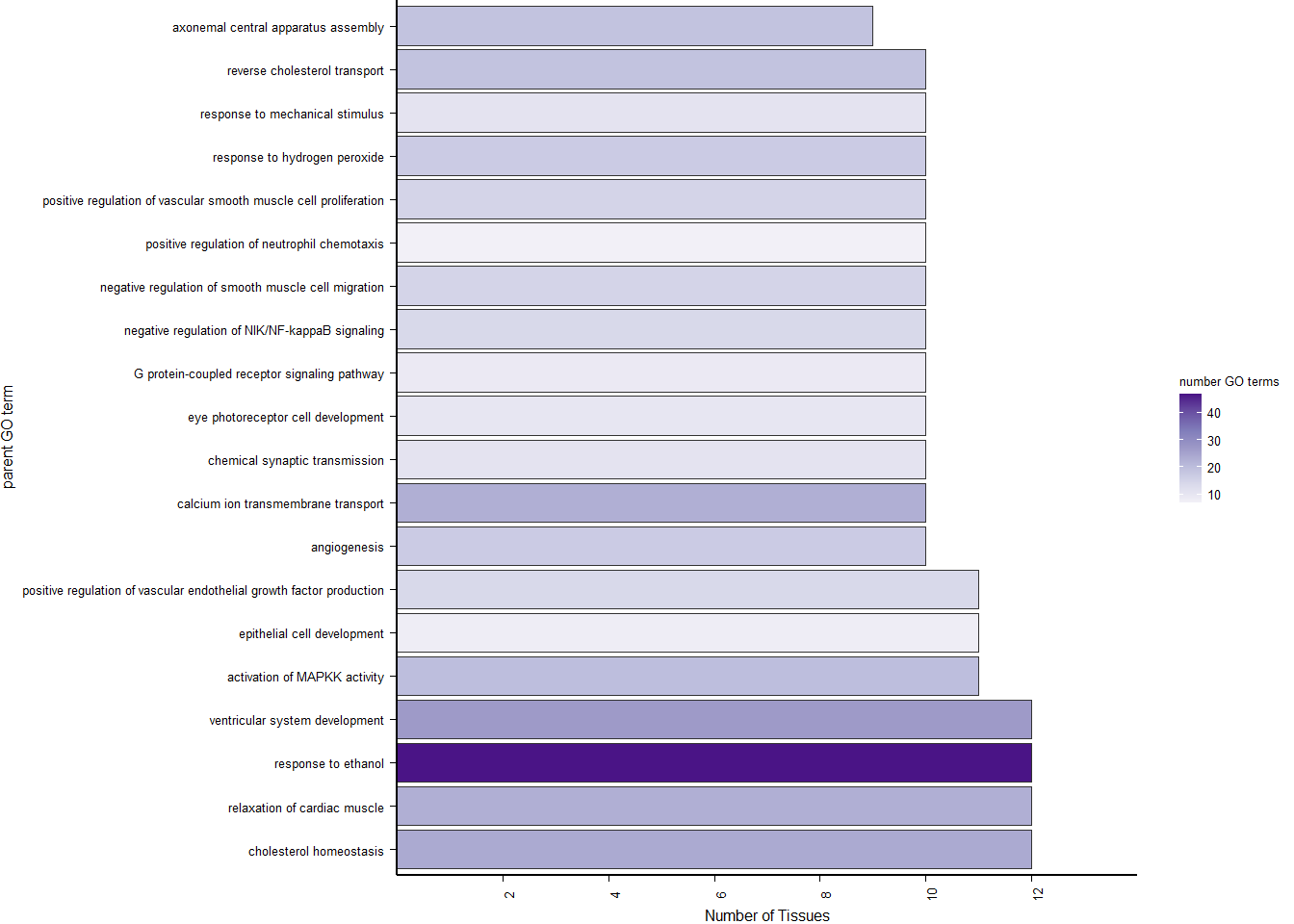
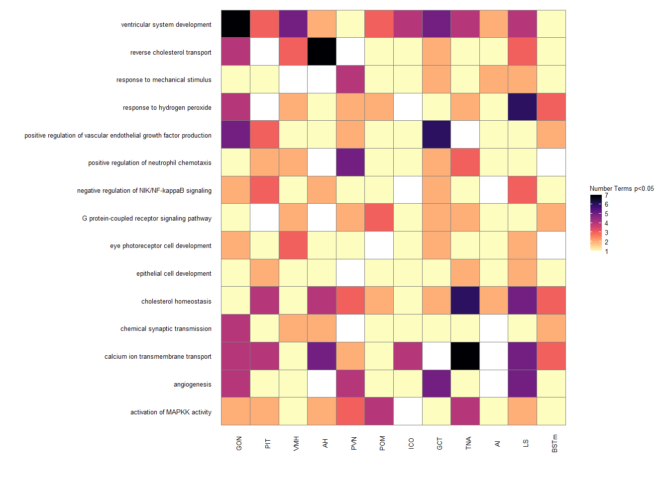
1.5 GO Overlap